Entropy
What is entropy
What does your desk look like right now?
If you are like most people, the honest answer is “worse than last week.” Not because you trashed it on purpose. Quite the opposite, you have been tidying up. But disorder is the default direction. Left alone, things drift toward mess.


That intuition is more precise than it feels. Behind it sits a mathematical structure that spans thermodynamics and information theory, and that structure is directly connected to a parameter you adjust every time you call an LLM.
Boltzmann’s desk
In the 1870s, Ludwig Boltzmann was chewing on a question that sounds easy until you try to answer it: why does heat always flow from hot objects to cold ones, never the other way around?
His answer was disarmingly simple: it is not that reverse flow cannot happen. It is just overwhelmingly unlikely.
Go back to your desk. Say there are five books, three pens, and a mug of coffee on it. “Tidy” configurations are rare: books sorted by size, pens in the holder, coffee safely to the right of the keyboard. “Messy” configurations are legion. Books at every angle, pens in every crevice, coffee perched ominously above the trackpad. The number of ways to be messy dwarfs the number of ways to be neat.
Boltzmann compressed this into a single line:
is entropy. is the number of microscopic arrangements that all look the same from the outside, the count of microstates compatible with a given macrostate. A tidy desk has a small , so low entropy. A messy desk has an enormous , so high entropy.
Systems drift from low- states toward high- states without anyone pushing them, purely because high- states occupy a vastly larger share of possibility space. That is the statistical heart of the second law of thermodynamics. Not a prohibition. A crushing probability.
Shannon’s telephone line
In 1948, Claude Shannon was sitting in Bell Labs working on an entirely different problem: how do you quantify how much information a communication channel can carry?
He needed a measure for surprise. “How uncertain was I before I received this message?” The more uncertain you were, the more information the message carries. “The sun will rise tomorrow” tells you almost nothing. “There will be a total solar eclipse tomorrow” tells you a great deal.
The formula Shannon arrived at:
is information entropy. is the probability of the -th possible outcome. When all outcomes are equally likely, is at its maximum: you have no basis for predicting what comes next. When one outcome’s probability approaches 1, drops toward zero. The result is a foregone conclusion, carrying no surprise at all.
Two people, different fields, different decades, facing different problems, arrived at structurally identical formulas.
Not a coincidence. In 1957, E.T. Jaynes provided the unifying framework: Boltzmann’s physical entropy and Shannon’s information entropy are instances of the same mathematical structure, a measure of uncertainty, or equivalently, of the number of states compatible with what you know. In physics it quantifies uncertainty over microstates; in information theory, uncertainty over messages. Same skeleton, different flesh.
There is an often-repeated anecdote about Shannon’s choice of the word “entropy” for his measure. Supposedly, von Neumann advised him to use the term, partly because the connection to thermodynamic entropy is genuine, and partly because “nobody really knows what entropy means, so in a debate you will always have the advantage.” Whether the story actually happened is anyone’s guess. But it has survived decades of retelling, probably because it captures something real about the concept: mathematically rigorous, intuitively slippery.
Temperature: the entropy knob you already use
If you have ever called an LLM API, you have adjusted a temperature parameter.
The name is not a metaphor. It does mathematically the same thing as the temperature parameter in the Boltzmann distribution.
When an LLM generates the next token, it first computes a raw score (logit) for every token in its vocabulary. Those scores then pass through a softmax function to produce a probability distribution, and temperature is the scaling factor in that conversion.
Set temperature close to 0 and the distribution collapses. The highest-scoring token absorbs nearly all the probability mass, output becomes near-deterministic, and in Shannon’s formula approaches zero.
Crank it up and the distribution flattens. The gap between high-scoring and low-scoring tokens shrinks, output grows unpredictable, entropy climbs. Push temperature toward infinity and the distribution converges to uniform; hits its maximum.
You are not “sort of like” controlling entropy when you move that slider. The Shannon entropy of the output distribution changes monotonically with temperature. Mathematical fact, not analogy.
The LLM softmax output is , where is the logit and is temperature. This is structurally identical to the Boltzmann distribution . As , the distribution degenerates to argmax (zero entropy); as , it converges to uniform (maximum entropy). Shannon entropy is strictly monotonically increasing in — not an empirical observation, but a mathematical property of the softmax function.
In physics, high temperature means particles explore their microstates more randomly. In an LLM, high temperature means the model explores its token space more randomly. Same formula, same behavior, different substrate.
From your desk to agent systems
Back to the desk.
A tidy desk has few compatible states, low entropy. But you do not need to do anything special to make it messier. You just need to use it. Every book you pick up, every pen you set down, every sip of coffee nudges the system toward higher entropy. Maintaining low entropy costs continuous energy: you have to keep tidying.
A long-running agent system faces the same force. Context windows accumulate noise. Tool calls inject unpredictable external state. Intent drifts across multi-turn conversations. Errors cascade and amplify. None of these are bugs. They are the default direction.
But “an agent system’s desk is getting messier” is, so far, just an intuition. To turn it into something with engineering weight, several questions need answers. What exactly is the “desk” in an agent system? What counts as “messy”? How fast does the mess grow? And can any of it be measured?
Further reading
- Shannon, C.E. (1948). “A Mathematical Theory of Communication.” Bell System Technical Journal, 27(3), 379-423.
- Jaynes, E.T. (1957). “Information Theory and Statistical Mechanics.” Physical Review, 106(4), 620-630.
Entropy in agent systems
Say your agent has been running for two hours. You come back and check the results. What it produced isn’t wrong, exactly — but it’s off. The direction shifted. Details warped. Some decisions are baffling.
You try to trace backward: where did it go sideways? There’s no clean turning point. No single catastrophic mistake. It’s more like a river that quietly changed course while you weren’t watching — each meter of drift negligible, and two kilometers later you’re in a different valley.
This isn’t a one-off. It’s the shared fate of every long-running agent system.
Understanding why it happens requires pulling apart three distinct phenomena.
Three degradations
Context rot — the signal is drowning.
The longer an agent runs, the more its context window accumulates: prior conversations, tool call returns, intermediate reasoning traces, file content summaries. As context grows, the model’s attention to any single piece of information thins out. Chroma’s experiments measured this precisely: the same critical fact, accurately retrievable from 100 tokens of context, starts losing fidelity at 10,000 tokens. The task didn’t get harder. The signal got buried.
Worse, not everything in the context is useful. Abandoned approaches, early wrong hypotheses, stale intermediate states. They sit in the context like noise, interfering with retrieval of what actually matters. Chroma’s data shows this interference is uneven, and the unevenness amplifies as context length grows.
Error cascade — mistakes are compounding.
In multi-step tasks, a small error in step one changes the input conditions for step two. A wrong function signature in the first step means the second step sees an interface that looks plausible but is semantically broken. It doesn’t know the interface is wrong. It reasons forward from a false premise, producing output built on a rotten foundation.
If steps were independent, 95% per-step success over ten steps gives you roughly 60% end-to-end. Geometric decay, unpleasant but predictable. Observed decay is faster. The SWE-EVO benchmark extends single-issue code fixes into multi-step software evolution: same kind of task, but the step count climbs from under 2 PRs to nearly 15. Even the strongest model-framework combinations solve only 25%, and 64% of tasks defeat every combination tried. These same model families score above 70% on single-step fixes. ReliabilityBench data confirms the super-linear pattern from another angle: inter-step errors are positively correlated. One step failing makes the next step more likely to fail, not less.
This isn’t the trivial explanation of “do more, break more.” It’s coupled amplification: each error doesn’t just fail on its own terms; it poisons the input to whatever comes next.
Intent drift — behavior detaches from purpose.
You ask it to refactor a module; midway through, it starts adding comments to unrelated files. You ask it to fix a bug; it starts “incidentally optimizing” surrounding code. There’s no visible fracture. Each individual step has a certain logic to it. But the overall heading is quietly rotating, and the final output sits at a strange distance from what you originally asked for.
Three degradations, three names. At first glance, three independent problems calling for three independent solutions.
It isn’t that simple.
Not three problems
Run a counterfactual.
Start by removing context rot. The model’s attention over 100,000 tokens is as uniform and precise as over 100. No signal dilution at all. Does error cascade vanish? No. A wrong output in step one still corrupts step two’s inputs; coupled amplification still happens. And as long as error cascade is present, the agent’s behavior will gradually diverge from intent through accumulated errors. Drift remains.
Now remove error cascade. Every step runs on fully correct preconditions, with zero inter-step coupling. Does context rot vanish? No. Context still accumulates, attention still thins, interference still interferes. And as long as context rot is present, the model’s ability to retrieve what matters degrades over time, and its grasp on “what am I actually supposed to be doing” gets fuzzier. Drift remains.
Finally, suppose intent drift itself were perfectly eliminated. The agent’s behavior stays laser-locked on the original intent, zero deviation. Context rot does not vanish; context is still bloating, attention still diluting. Error cascade does not vanish; coupled amplification in multi-step tasks has nothing to do with whether intent stayed aligned.
Three counterfactuals, one clear conclusion:
- Eliminate context rot → drift is reduced, not eliminated
- Eliminate error cascade → drift is reduced, not eliminated
- Eliminate drift → context rot and error cascade proceed unchanged
Context rot and error cascade each independently produce drift. Drift’s elimination doesn’t touch either of them. Drift is effect, not cause.
Causal structure
The relationship between the three isn’t parallel. It has direction:
Context rot ──────→ Intent drift ←────── Error cascade
     ↑                                        │
     └────────────────────────────────────────┘
                  positive feedback loop
Context rot and error cascade are two independent degradation mechanisms, each driving intent drift through a different pathway. Drift is their emergent effect — once context signal is sufficiently diluted, or errors have sufficiently accumulated, the agent’s behavior must diverge from intent.
But there’s a loop in the diagram.
Errors from the cascade — wrong tool call results, wrong intermediate reasoning, wrong code edits — all get written into the context. They become the most dangerous category of noise in context rot: information that is highly relevant to the current task but factually wrong. In subsequent steps, the model works inside a context contaminated by its own mistakes. Attention isn’t merely thinned; it’s actively misdirected.
This loop couples the two independent mechanisms into a positive feedback system: cascade errors accelerate rot, worsening rot makes the model more error-prone on the next step, and the additional errors further contaminate the context. ReliabilityBench data offers indirect evidence for this feedback loop: the more sophisticated Reflexion architecture (reflect-then-retry) actually degrades faster than plain ReAct under fault injection, with failure recovery rates of 67.3% vs. 80.9%. The mechanism is the loop: the reflection layer extracts “lessons” from a poisoned context, the lessons themselves are wrong, and then wrong lessons guide the next action. The intent behind reflection is sound, but it adds an extra iteration to the feedback loop.
The information-theoretic view
These three phenomena have different names and different surface behaviors, but they share a common underlying language: information theory.
Model the agent system as a communication channel. The user’s intent is the signal source. The agent’s final behavior is the receiver. Every processing step in between (context retrieval, reasoning, tool invocation) is part of the channel.
Context rot is rising channel noise. Longer context means a lower signal-to-noise ratio. The original intent signal is diluted by growing volumes of irrelevant information and active interference. This is the fundamental problem in communication engineering: the longer the channel and the more noise it accumulates, the weaker the receiver’s ability to reconstruct the original signal.
Error cascade is noise compounding across cascaded channels. A multi-step task is a series of channels chained end-to-end. Each channel introduces some noise. That noise doesn’t simply stack; it compounds super-linearly, because each channel’s output noise becomes part of the next channel’s input noise. The perturbation amplifies as it propagates. The empirical evidence (positively correlated inter-step errors, success rates decaying faster than geometric models predict) is the statistical fingerprint of noise compounding.
Intent drift is the observable signal distortion. It isn’t a separate degradation mechanism. It’s the measurement at the receiver: the discrepancy you see when you compare the agent’s final behavior against your original intent. Channel noise (rot) and cascaded compounding (cascade) are the causes of distortion. Drift is the distortion itself.
This unification isn’t just rhetorical analogy. It carries a substantive implication: since all three phenomena are fundamentally noise problems in an information channel, the analytical framework for confronting them is the same. Understand how information degrades inside an agent system, and you hold a single lens for examining every form of degradation.
The full landscape is in view: two independent mechanisms, one emergent effect, one positive feedback loop. But a landscape is not a map of the terrain underfoot. To understand how each mechanism actually unfolds inside an agent, you need to go closer.
What are the specific degradation modes of context rot? How does attention dilution progress, step by step, toward signal loss? That’s the next question. And how exactly does error cascade’s coupled amplification work, why is it worse than what independent probability models predict? That’s the one right after.
Context rot
In 2026, mainstream models offer context windows of 256K to 1M tokens. Capacity is no longer the bottleneck — a two-hour agent session’s worth of tool call results, file contents, and conversation history fits comfortably. But the question was never about fitting. The question is: at token 500,000, how much does the model still “remember” about that critical instruction written back at token 1,000?
The intuitive answer is “as long as it hasn’t hit the window limit, everything is fine.”
That intuition is wrong.
Not an overflow, a dilution
Most engineers carry a mental model of the context window as a bucket. Pour water in; when it overflows, you lose something. As long as the bucket isn’t full, you’re safe. Under this model the only context-management problem is capacity, so 128K is better than 32K, 256K is better than 128K, 1M solves everything.
Chroma Research’s 2025 systematic study of 18 frontier LLMs tells a different story. They found that model performance degrades measurably as input token count grows. Not by hitting some cliff, but by declining continuously from the start. The window is nowhere near “full,” and performance is already sliding.
A better mental model: a cup of tea. The first few thousand tokens are strong brew. High signal density, sharp attention on every token. Then you keep adding hot water without adding tea leaves. Total liquid volume goes up. Concentration goes down. The cup never overflows. The tea becomes too weak to taste.
Chroma named this phenomenon context rot. Not overflow. Decay.
Three degradation mechanisms
Chroma’s experimental methodology deserves attention: they held task difficulty constant and varied only input length, isolating “input length itself” as the variable driving performance degradation. This control allowed them to separate three independent mechanisms.
Attention dilution. The Transformer’s self-attention mechanism has every token attend to every other token. When context grows from 1,000 to 100,000 tokens, the attention budget gets spread across 100x more positions. Experiments showed that when the semantic similarity between the needle (target information) and the question is low, this dilution becomes especially destructive. Not because the task got harder (the same needle-question pair performs well in short context), but because the model can no longer find its way through the sea of tokens.
Distractor interference. Tokens in the context that are topically related to the target but factually incorrect (distractors) actively mislead the model. Even a single distractor measurably degrades performance; four distractors make it worse. What caught Chroma’s attention: different distractors interfere with unequal strength, and this unevenness amplifies as input length grows.
There is also a counterintuitive divergence in how different model families break. Claude-family models tend toward abstention: “I can’t find a confident answer, so I won’t answer.” GPT-family models tend toward confident response, even when the answer comes from a distractor rather than the needle. One chooses false negatives; the other chooses false positives. Same degradation pressure, different failure modes.
Structural interference. This is the most counterintuitive of the three. The experiments found that a logically coherent, well-structured haystack (background text) actually damages needle retrieval performance more than a haystack with sentences randomly shuffled.
Why? One hypothesis: the attention mechanism gets “captured” by structured content. A coherent passage has stronger local correlations. Sentences reference each other, paragraphs build on one another, and these correlations siphon attention away from the needle. Shuffle the sentences, break the local coherence, and attention is freed up to find the needle more easily.
Think about what this means for agent systems. Your carefully formatted tool outputs, your cleanly structured file contents, your logically coherent conversation history. The “good engineering practices” that produce well-organized context may be competing with your core instructions for the model’s attention at the mechanism level. The effort you spend making context more orderly might be making it harder for attention to find the one instruction that matters.
Lost-in-the-Middle is only one facet
If you have followed long-context research, you have probably encountered Liu et al.’s 2024 “Lost in the Middle” finding: models retrieve information worst from the middle of their context, producing a U-shaped curve. Beginnings and endings are remembered, middles are forgotten.
That finding is real, but it describes only one slice of context rot: positional bias. Chroma’s experiments, testing across 11 needle positions, found no significant positional effect. The degradation they observed depended not on where information was placed, but on how long the context was, how many distractors it contained, and how structured the content was.
In other words, Lost-in-the-Middle is a special case of context rot, not the whole picture. You can mitigate positional bias by placing critical information at the start or end. You cannot mitigate attention dilution, distractor interference, or structural interference by rearranging positions. These are deeper sources of decay.
Maximum Effective Context Window
The three mechanisms point to a practical concept: Maximum Effective Context Window (MECW), the actual context length at which a model can maintain reliable performance on a given task.
MECW is far smaller than the advertised window size. Paulsen’s 2025 testing on real-world tasks showed that some frontier models begin failing at roughly 100 tokens of input, with most showing clear accuracy degradation by 1,000 tokens — far below their advertised limits. The gap between advertised and effective window can be orders of magnitude.
And MECW is not a fixed number. Multi-step reasoning is more sensitive to context quality than single-step retrieval, so the same model’s MECW can vary by orders of magnitude across tasks. The signal-to-noise ratio in context keeps shifting; more noise, smaller MECW. Distractor density keeps shifting; topically related but incorrect content is the most lethal form of noise. Even the degree of structural organization matters. Structural interference means well-organized context is not necessarily friendlier than messy context.
Chroma’s experiments used minimal tasks: find a fact in a text, answer a question. Real agent tasks involve multi-step reasoning, tool calls, state tracking, all far more complex than needle-in-a-haystack. In real agent scenarios, MECW is almost certainly smaller still.
A channel-capacity lens
Attention dilution, distractor interference, structural interference. Three mechanisms that look independent, but they share an underlying structure. Shannon’s channel capacity formula helps make it visible:
is channel capacity (the maximum rate at which information can be reliably transmitted), is bandwidth, and is the signal-to-noise ratio.
Think of the context window as a channel. is window size, how many tokens you can fit. is the ratio of signal tokens to noise tokens in the context. is the amount of useful information the model can actually extract.
This analogy is not a mathematical equivalence. A context window is not a memoryless Gaussian channel, and the attention mechanism is not a linear decoder. But the formula captures the structural essence of context rot:
Increasing cannot raise without bound, because is falling in tandem.
Every agent loop that dumps material into context (raw tool outputs, complete file contents, fragments of intermediate reasoning) is mostly noise or weak signal. The window gets bigger, but the signal-to-noise ratio deteriorates. The spirit of Shannon’s formula: as approaches zero, approaches zero regardless of how large is.
This is why “solve context rot with a bigger context window” is a self-defeating strategy. You widen the pipe, but you pump more noise through it.
And it is why Chroma’s three mechanisms feel natural under this framing: attention dilution is the passive decline of as grows; distractor interference is the active increase of (topically related but incorrect content is the most effective noise); structural interference is the special case where signal gets masked by structured noise.
Can context rot be “fixed”? It can — but the fix lives at the model layer, not the harness layer. How to maintain uniform attention across long sequences, how to reduce distractor interference, how to prevent structured content from hijacking attention — these are problems for model researchers, squarely within the force described in ch-01. From Sparse Attention to Ring Attention to various long-context architectural innovations, model-level progress keeps pushing the MECW ceiling higher.
But harness engineers work with the models that exist today. Given a model’s current attention characteristics, what the harness controls is signal-to-noise ratio — what enters the context, what stays out, when to compress, how to compress. This is channel engineering, not channel physics.
Recognizing which layer owns which problem saves you from pushing in the wrong place. The entropy story always has two halves: one about disorder growing, the other about what you can do within the constraints. While context decays, the agent keeps making decisions, calling tools, producing outputs. Every diluted instruction, every misdirected retrieval, can push the next step further off course. Degradation does not sit still. It flows.
Further reading
- Chroma Research (2025). “Context Rot: How Increasing Input Tokens Impacts LLM Performance.”
- Liu, N.F. et al. (2024). “Lost in the Middle: How Language Models Use Long Contexts.” TACL.
- Paulsen (2025). “The Maximum Effective Context Window for Real World Tasks.”
Error cascade
Here is a math problem.
An agent succeeds at each step with 95% probability. Ten steps in a row. If each step is independent, the overall success rate is .
That alone should set off alarms — a system that looks rock-solid on any single step drops to a coin-flip-plus-change over ten. But the number assumes something very specific.
In the real world, the number is lower than 60%. Sometimes much lower.
Compound interest in reverse
Let’s make the assumption explicit. The calculation treats each step as independent: whether step three succeeds has nothing to do with what happened at steps one and two. Like coin flips: the last toss doesn’t know about the one before it.
Under this model, multi-step reliability decays geometrically. Each additional step multiplies the running total by the same factor. Compound interest grows wealth exponentially; geometric decay shrinks reliability at the same relentless rate.
Even this “optimistic” model is sobering. At 95% per step: 20 steps gives you . Fifty steps, .
But geometric decay is the gentle scenario. It is the mildest possible multi-step decay curve, because it assumes zero information transfer between steps. Each step faces a clean slate, uncontaminated by its predecessors.
In real agent tasks, that assumption almost never holds.
Beyond probability multiplication
The independence assumption says each step encounters a problem state untouched by prior results. But in multi-step agent work, the output of one step is the input of the next. Steps are not independent dice rolls — they share state.
This coupling breaks independence through at least three channels.
Interface contamination. A code-modification agent changes a function signature at step one. The change is wrong: the parameter types pass static checks, but the semantics have shifted. Step two calls that function and sees a perfectly legal-looking interface with silently incorrect behavior. Nothing signals a problem. Step two’s failure probability is no longer an independent 5%; it has been inflated, invisibly, by step one’s error.
Test signal masking. A prior step introduces a regression. Subsequent steps run the test suite and see failures. But the agent cannot distinguish which failures it just caused from which were already there. The test signal — the primary error-correction mechanism — is drowned in noise. This is not merely “harder to succeed.” It is “the correction machinery itself has been degraded.”
Context drift. In long-running sessions, flawed reasoning from earlier steps gets written into the context window. Later steps reason on top of that contaminated context. The model does not spontaneously question things “it said earlier.” It tends to continue along the established trajectory rather than stepping back to audit the entire chain. Once a false assumption enters the context, it replicates into every downstream step like a mutation copying through cell division.
Three channels, one shared consequence: a prior step’s error does not simply add an independent failure probability to the next step. It changes the problem the next step is solving.
What the benchmarks show
Theory says “worse than geometric.” How much worse?
SWE-EVO (2025) extends code repair from single issues to multi-step software evolution: consecutive modifications to the same repository, spanning multiple PRs, cross-file dependencies, and escalating complexity. The results speak plainly: task difficulty scales with PR count (averages of 1.67, 3.57, 6.71, and 14.84 PRs across difficulty tiers), even the strongest model-framework combination solves only 25%, and 64% of tasks defeat every combination tried. These same model families score above 70% on single-step fixes (SWE-Bench Verified). Same code-editing capability, stretched across more steps, and performance falls off a cliff.
Beyond pass@1 (2026) quantifies this super-linear decay from a different angle. They directly measure inter-step error correlation and find , meaning once an agent drifts onto the wrong path, it tends to stay there rather than self-correcting. Qwen3 30B posts a short-task pass@1 of 75.8%; geometric decay predicts roughly 33% on long tasks; the actual figure is 22.2%, a 1.5x gap. Mistral Nemo’s gap is sharper: predicted 28.6%, actual 12.1%, a 2.4x shortfall. Formally, positively correlated errors push task failure probability from to , a super-exponential function of .
| Model | Short-task pass@1 | Geometric prediction | Actual long-task | Gap |
|---|---|---|---|---|
| Qwen3 30B | 75.8% | ~33% | 22.2% | 1.5x worse |
| Mistral Nemo | — | 28.6% | 12.1% | 2.4x worse |
ReliabilityBench (2026) surfaces a counterintuitive finding: under fault injection, the more sophisticated Reflexion architecture (reflect-then-retry) degrades faster than plain ReAct, with a fault recovery rate of 67.3% versus 80.9%. The mechanism: Reflexion’s reflection layer tries to extract “lessons” from erroneous tool returns, but those lessons are themselves built on bad data. Applying a false lesson to the next step is context drift instantiated at the architecture level. The longer the reasoning chain, the greater the amplification when any single link in that chain is compromised.
The data converge on a single conclusion: multi-step agent reliability decays super-linearly, rooted in positive inter-step error correlation.
The positive feedback loop
Error cascade does not operate in isolation. It forms a positive feedback loop with context rot.
One step’s error contaminates the context — bad reasoning traces, incorrect intermediate results, false assumptions. The contaminated context weakens subsequent steps’ ability to self-correct; the model reasons through noise and is more likely to err. More errors produce more context contamination. More contamination further degrades correction capacity.
These are not two independent degradation processes that happen to coincide. They feed each other. Error cascade accelerates context rot; context rot accelerates error cascade. Positive feedback means that past a certain tipping point, degradation becomes self-sustaining. No external perturbation required, the system drifts on its own.
GLM-4.5 Air’s data is a direct fingerprint of this loop: on short tasks, only 1% of episodes terminate before the first subtask even begins. On extra-long tasks, that figure rises to 25%. Early-termination rate increases monotonically with task length, meaning the cumulative errors from prior steps are not just making later steps “harder.” They are eroding the system’s capacity to even begin attempting the next step.
Complexity as amplifier
The severity of cascade is not a constant. It depends heavily on the degree of coupling between steps.
Beyond pass@1 stratified their measurements by task domain, and the differences are stark:
| Domain | Short-task success | Extra-long success | Decay |
|---|---|---|---|
| Code editing (SE) | 0.90 | 0.44 | -0.46 |
| Web research (WR) | 0.80 | 0.63 | -0.17 |
| Document processing (DP) | 0.74 | 0.71 | -0.03 |
Code editing is catastrophic, from 90% down to 44%, nearly halved. Document processing barely moves: 74% to 71%, within noise.
The difference is coupling.
Code modification is a tightly dependent multi-step process. Every line changed can affect the correctness of every subsequent step. Alter a function signature and every call site must follow; restructure a data type and all read/write logic must synchronize. A single error propagates along the dependency graph to every downstream step. This is fertile ground for interface contamination and test signal masking.
Document processing is weakly dependent. Extracting a table from page three and a paragraph from page seven share almost no state. Getting one wrong does not affect the other. Steps exchange minimal information, and errors have no propagation path.
Same model. Same number of steps. Radically different decay curves. What determines cascade severity is not the step count itself, but the coupling between steps. Step count merely provides opportunity for cascade; coupling determines how thoroughly each opportunity is exploited.
ReliabilityBench’s reliability surface confirms this from another dimension: the degradation gradient along the fault-tolerance axis () is steeper than along the robustness axis (). Infrastructure faults (timeouts, rate limits) trigger cascade more readily than input perturbations like phrasing changes, because infrastructure faults attack the state-transfer channels between steps directly. They are assaults on the coupling itself.
Error cascade is a thermodynamic-grade force. It is the default direction — you do not need to do anything wrong for it to operate. You only need enough steps and enough coupling between them.
Is there any way to push against this default direction? Physics has a classic thought experiment for that question: Maxwell’s Demon — a tiny guardian who can observe the state of every molecule and intervene with precision. But Maxwell himself knew the demon does not work for free. Opposing entropy has a price. The structure of that price is worth examining.
Further reading
- SWE-EVO (2025). Can LLM Agents Maintain a Clean Codebase? arXiv:2512.18470.
- Beyond pass@1 (2026). A Reliability Science Framework for LLM Agent Systems. arXiv:2603.29231.
- ReliabilityBench (2026). Evaluating LLM Agent Reliability Under Production-Like Stress Conditions. arXiv:2601.06112.
Maxwell’s Demon
In 1867, James Clerk Maxwell imagined a creature.
It sits by a tiny door in a partition dividing a gas container. It can tell fast molecules from slow ones. Fast ones go left, slow ones go right. No work performed, yet heat flows spontaneously from cold to hot. The second law, defeated.
Or so it seemed.
The thought experiment has outlived Maxwell by more than a century and a half. It persists not because it is clever, but because it encodes a structural fact: information and physical order have an exchange rate.
That fact happens to be an exact description of what harness engineers do every day.
What the Demon does
The setup, stated precisely.
An insulated container. A partition in the middle. A door in the partition. Gas molecules bounce around on both sides. The Demon watches each molecule that approaches the door. Slow molecule on the left side? Open the door, let it through to the right. Fast molecule on the right? Open the door, let it through to the left. Otherwise, keep the door shut.
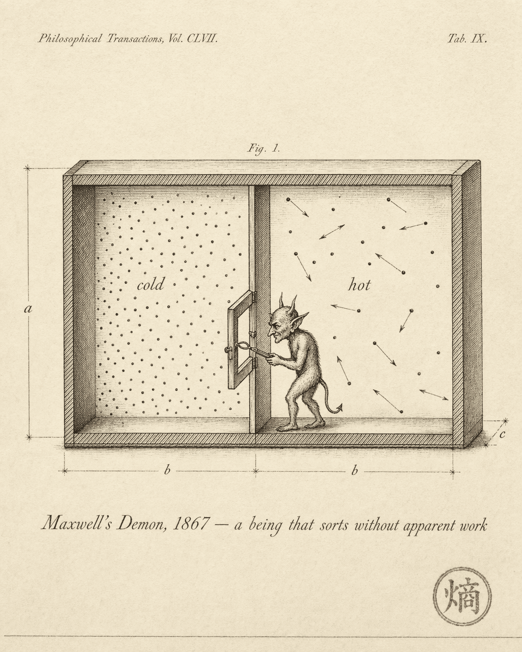

After enough rounds, the left side holds only fast molecules (high temperature), the right side only slow ones (low temperature). A uniform-temperature system has been sorted into a hot half and a cold half. Entropy has decreased.
No work was done. The door is massless; opening and closing it costs effectively nothing. The second law says entropy in an isolated system can only increase or stay the same. The Demon appears to violate it.
This paradox stood unresolved for over a hundred years.
Information is not free
The answer arrived in two stages.
In 1961, Rolf Landauer at IBM made a claim that looked modest at first: erasing one bit of information produces at least of heat. This is not an engineering limitation. It is a physical law. Destroying information is an irreversible physical process, and irreversible processes necessarily generate entropy.
In 1982, Charles Bennett connected Landauer’s principle back to Maxwell’s Demon. To sort molecules, the Demon must complete a full information-processing cycle:
- Measure: observe a molecule’s velocity, acquiring information.
- Decide: based on that velocity, open or keep shut.
- Store: record the decision (without memory, it cannot sustain operations).
- Erase: when storage fills up, clear old records to make room.
Steps 1 through 3 can, in principle, be designed as thermodynamically reversible, generating no extra entropy. Step 4 cannot. Landauer’s principle is unambiguous: erasure is irreversible. Every bit of cleared memory dumps at least of heat into the environment.
The Demon reduces entropy inside the container, but increases entropy in itself and the environment through information erasure. When you settle the full account, the second law holds — not a scratch on it.
Order does not appear from nothing. The cost of sorting is hidden in the final step of information processing.
Earman & Norton have long questioned the sufficiency of the Landauer-Bennett resolution, and a 2025 paper (arXiv:2503.18186) further argues that measurement, not erasure, is the step where entropy is truly generated. The debate remains open. But regardless of which step carries the cost, the core conclusion is untouched: sorting information cannot be free. The only question is which line item the bill lands on.
The mapping
What a harness engineer does and what the Demon does are structurally the same operation. The correspondence is tighter than metaphor: it is a structural mapping.
| Demon’s world | Harness engineer’s world |
|---|---|
| Gas molecules | Tokens, tool outputs, external data |
| Distinguishing fast from slow | Filtering, validation, routing |
| Opening / closing the door | Selectively injecting or blocking information into the context window |
| Storing records | The context window itself |
| Erasing old records | Compaction, summarization |
The Demon sorts molecules to reduce thermodynamic entropy in the container. The harness engineer sorts information to reduce information entropy in the system, keeping the context window high-signal and low-noise, making the agent’s next action as deterministic and correct as possible.
This is not a coincidence of analogy. Return to the framework from the first article in this chapter: information entropy and thermodynamic entropy share the same mathematical skeleton. On that skeleton, the Demon’s operations and the harness engineer’s operations occupy isomorphic positions.
And isomorphism means the constraints are isomorphic too.
The cost of sorting
Landauer’s principle exacts its toll in heat. In agent systems, the toll takes different forms, but the structure is identical: every operation that reduces information entropy carries an irreducible cost.
To be clear: the mapping is structural, at the information-theoretic level. Compaction does not literally generate heat. In the physical world, the cost is thermal dissipation. In agent systems, it is information loss, computational expense, and complexity growth. Different currencies, same ledger.
Start with compaction. Compressing conversation history inevitably discards detail. Factory’s research, tested across more than 36,000 real development session messages, surfaced a stark number: every compression scheme scored only 2.19 to 2.45 out of 5.0 on artifact tracking (the ability to maintain awareness of file changes). No matter how carefully you design a structured summary, compression loses things. If those lost details are needed later, the agent must re-acquire them, and the tokens saved may not cover the bill for re-acquisition.
Validation has its own bill: latency and tokens. Every check on a tool’s output, every verification of an LLM’s response, consumes compute and time. Stricter validation means a bigger bill.
Routing pays in complexity. Dispatching tasks to different subsystems or sub-agents requires routing logic, edge case handling, state synchronization. Every additional layer of sorting adds a layer of cognitive overhead to the system.
None of these costs indicate poor implementation. They are structural. The Demon cannot reduce entropy in the container without increasing entropy in the environment. A harness engineer cannot maintain system order without paying a price.
There is no free order maintenance.
The entropy control philosophy
This chapter has followed a single thread. It started with the mess on your desk, passed through Boltzmann’s microstate counting, Shannon’s information measure, the dual identity of the temperature parameter, and arrived here — at Maxwell’s small creature and the information cost it cannot escape. All of it points at the same conclusion.
Entropy increase is the default direction. Opposing it requires a cost. That cost is irreducible. You can manage it. You cannot eliminate it.
This is the entire philosophy of entropy control: not the pursuit of zero entropy, but the search for the optimal operating point under the constraint of entropy increase.
Zero entropy is an illusion. An agent system that chases “never wrong,” “context never degrades,” “information never lost” will watch its costs balloon past any reasonable budget. Infinite validation layers, infinite context windows, infinite redundancy. It is the equivalent of keeping your desk in first-day condition while actively using it: theoretically possible, practically meaning you spend all your time tidying and none working.
But abandoning order is not an option either. An agent system that does no information sorting — no compaction, no output validation, no noise filtering — loses coherence rapidly under entropy increase. The research on context rot has quantified this: even with very large context windows, accumulated information itself degrades model performance.
The optimal operating point sits somewhere between those extremes. It depends on task characteristics, model capability, acceptable failure rates, tolerable latency, and budget. It is not a fixed point. It is a balance that requires continuous adjustment.
Entropy control is not a technique, a framework, or a checklist. It is a design philosophy: acknowledge that costs exist, then make choices within the constraints.
The Demon cannot abolish the second law of thermodynamics. What it can do is understand where the costs lie, and decide whether each bill is worth paying.
If entropy control is the philosophy, then applying it across an agent system’s full lifecycle (from context curation to error recovery to long-running operation) demands something beyond a single Demon’s intuition. It demands a systematic engineering methodology.
Further reading
- Landauer, R. (1961). “Irreversibility and Heat Generation in the Computing Process.” IBM Journal of Research and Development, 5(3).
- Bennett, C.H. (1982). “The Thermodynamics of Computation — A Review.” International Journal of Theoretical Physics, 21(12).
- Factory.ai (2025). “Evaluating Context Compression for AI Agents.”
Engineering under the Second Law
Cybernetics tells you what feedback loops look like. Entropy tells you why they exist. Two stories — but they are two sides of the same story.
The previous articles mapped out how entropy manifests in agent systems: context rot dilutes signal, error cascades amplify noise, the two couple into positive feedback that drives intent drift. The full picture is clear. But it only answers “what happens.” It does not answer a more fundamental question: in a system where entropy always increases, is reliable engineering even possible?
In 1948, Claude Shannon gave a surprisingly optimistic answer.
The channel coding theorem
In his landmark paper, Shannon proved something counterintuitive: on a noisy channel, as long as the transmission rate stays below the channel’s capacity , there exists an encoding scheme that can push the error rate arbitrarily close to zero.
The power of this theorem is not in telling you how to encode. It is an existence proof: fighting noise does not require infinite energy — it requires the right structure.
Noise cannot be eliminated. Channel capacity is a hard constraint. But within that constraint, systematic encoding lets the signal pass through noise and arrive at the other end nearly intact.
A necessary qualification: agent systems are not the discrete memoryless channels Shannon’s math describes. An agent’s “noise” has memory, structure, temporal correlation; the superlinear decay in error cascades is direct evidence that successive errors are not independent. Shannon’s specific equations do not port over. But the structural insight (that operating space exists within constraint, and that redundancy and verification are the mechanisms that unlock it) reaches far beyond its original proof.
Two kinds of coding
Shannon’s framework splits the encoding problem into two halves, each solving a different problem.
Source coding strips away redundancy. Raw signals from any source contain predictable structure: in English text, the letter ‘e’ appears far more often than ‘z’; adjacent pixels in an image are almost always similar. Source coding exploits that predictability to represent the same information in fewer bits. The core operation is compression.
Channel coding adds structured redundancy back in. After compression, the lean signal is fragile; a single bit flip can cause unrecoverable damage. Channel coding deliberately introduces redundancy: check bits, error-correcting codes, repeated transmissions. This redundancy carries no new information, but it lets the receiver detect and correct errors introduced during transit. The core operation is verification and correction.
The two seem to pull in opposite directions (one removes redundancy, the other adds it), but they work together in the same system: compress down to the essential information, then protect that essential information with structured redundancy as it passes through the noisy channel.
| Dimension | Source coding | Channel coding |
|---|---|---|
| Operation | Strip redundancy / compress | Add structured redundancy |
| Harness equivalent | Compaction, summarization | Testing, validation, assertion |
| Goal | Represent core info in fewer tokens | Detect and correct execution errors |
Squint at what a harness does, and the isomorphism is striking.
Compaction is source coding. When the context window approaches its limit, compaction compresses conversation history, raw tool outputs, and intermediate reasoning into structured summaries, stripping away the predictable, the redundant, the stale, keeping only what matters. Factory’s anchored summarization, Anthropic SDK’s built-in compaction, OpenAI’s compact endpoint. Different engineering paths, same underlying operation: source coding.
Tests, type checks, assertions, output validation. These are channel coding. They produce no new functionality. A program that passes all its tests does not have a single line of business logic more than one without tests. But they inject structured redundancy that lets the system detect errors introduced during execution. Every green CI run is a successful decode: the signal passed through the noisy channel and the check bits confirmed it arrived undistorted.
The two kinds of coding cooperate inside the harness the same way they do in Shannon’s framework: compaction compresses context down to essentials; validation protects those essentials from being swallowed by noise across multiple execution steps. Drop the first, and context bloats until attention dilutes. Drop the second, and errors cascade with nobody watching.
Feedback loops as anti-entropy
The cybernetics chapter described four nested feedback loops: token-level, turn-level, session-level, alignment-level. The language was cybernetic: observer detects deviation, controller applies correction, negative feedback counteracts positive feedback.
Now put on a different lens.
The fastest loop is token-level. The autoregressive mechanism is itself a correction circuit: every token generated immediately becomes input conditioning the next. The model uses preceding output to calibrate subsequent generation on a millisecond timescale, essentially a channel decoder with an extremely short time constant, counteracting randomness in the token distribution.
One layer up, turn-level feedback operates on a scale of seconds to minutes. The model calls a tool; the tool returns a signal from the real world: file contents, test results, compilation errors. That signal gets spliced back into context and calibrates the next decision. Each tool call is one sample of external reality; each result returned is one injection of error-correction signal. Output parsing, result validation, sanity checks: all channel coding at this layer.
Higher still, session-level. After a session ends, CI results, user feedback, and progress-file diffs provide a coarser-grained check: not just “was this step correct” but “is the overall direction right.” Context resets, prompt template switches, tool-set adjustments: correction operations that counteract drift accumulated across many turns.
The slowest loop is alignment-level. Human preference signals altering model weights through training, on a cycle measured in weeks and months. It corrects not the deviation of a single output but systematic bias in the model’s probability distribution.
Four loops, four timescales, all counteracting the same thing: entropy increase. Fast loops catch small deviations before they amplify. Slow loops catch systematic bias before it calcifies. Cybernetics describes them as “nested Observer-Controller-Plant circuits.” Information theory describes them as “error-correction coding layers operating at different timescales.” Both descriptions point at the same structure.
Cybernetics and entropy are not two independent theoretical frameworks. Cybernetics describes the topology of feedback: what connects to what, how signals flow, how positive and negative feedback interweave. Entropy and information theory explain why those loops must exist, because a system’s default trajectory is toward disorder, and error correction is the only mechanism that maintains order. Topology and dynamics. Structure and rationale. Two sides of the same coin.
Ashby’s Law reread through information theory
When the cybernetics chapter introduced Ashby’s Law, the language was cybernetic: the controller’s variety must be no less than the variety of disturbances it needs to counteract. V(C) >= V(D).
Information theory offers a second reading.
What does “variety” measure? The number of possible states a system can occupy. And the logarithm of the number of possible states. That is entropy. Ashby’s variety and Shannon’s entropy are the same quantity in different notation.
The controller’s variety V(C) is the number of distinct control signals it can emit, i.e. the capacity of the control channel. The disturbance variety V(D) is the number of distinct perturbations the environment can impose, i.e. the bandwidth of the noise channel.
V(C) >= V(D), translated into information-theoretic terms: the capacity of the error-correction channel must be no less than the bandwidth of the noise channel. The controller needs enough channel capacity to transmit correction information; otherwise, some fraction of the noise “leaks” past the correction net. Whatever leaks through is the system’s blind spot.
Back in the harness context: the “noise bandwidth” an agent system faces (context rot rate, error cascade amplification factor, external environment uncertainty) determines how much “correction capacity” the harness needs to provide. Tool variety and precision, validation coverage and accuracy, feedback loop time resolution. These constitute the harness’s error-correction channel. Ashby’s Law says: if the correction channel’s capacity falls short, noise wins.
This also explains an observation from the end of ch-02: why simple harnesses often win. Not because simplicity has intrinsic magic, but because reducing the plant’s effective variety (structured output, tool constraints, task decomposition) is equivalent to narrowing the noise channel’s bandwidth. Once bandwidth narrows, a simple correction channel is enough to cover it. Correction capacity matched precisely to noise bandwidth, no more, no less. The optimum that both Ashby and Shannon would recognize.
Not fighting, but understanding
The Second Law of Thermodynamics is a constraint at the scale of the universe. Total entropy does not decrease. No engineering trick bypasses this; it is physical law.
But Shannon’s proof reveals a crucial operating space: the Second Law constrains total entropy, not local structure. Against the backdrop of total entropy increasing, you can build and maintain local order — at the cost of producing more disorder elsewhere. An air conditioner cools the room but heats the outdoors. A refrigerator preserves food but warms the kitchen. Maxwell’s demon could theoretically sort molecules, but Landauer’s principle says erasing the demon’s memory dissipates energy.
A harness does exactly this. Compaction lowers entropy locally in the context (compressing away redundancy and noise), but it consumes token budget and compute. Tests and validation detect and correct errors at the output boundary, but they consume execution time and compute cycles. Every feedback layer counteracts entropy locally, but maintaining those layers is itself system overhead.
The goal was never “zero entropy.” A zero-entropy agent system is a fully deterministic one — no uncertainty whatsoever, and therefore no flexibility. It degrades into a hardcoded script.
The real goal is a sustainable balance between the rate of entropy increase and the rate of error correction. Context rot rate, error cascade amplification: these define the entropic pressure the system faces. Compaction frequency and quality, validation coverage and precision, feedback loop response speed: these define the system’s correction capacity. When correction rate keeps pace with entropy rate, the system maintains a dynamic order over time, not static equilibrium, but a continuous expenditure of energy to sustain a low-entropy state.
Thermodynamics has a name for this: a dissipative structure. An open system far from equilibrium, maintaining order through continuous energy input.
From demon to operating system
Three chapters of threads can now converge.
Orthogonality decomposed two independent forces: model capability and harness engineering, each doing its own work. Cybernetics gave the skeleton: feedback loop topology, OCP role separation, Ashby’s variety constraint. Entropy gave the dynamics: why entropy increase is the default direction, how noise propagates and amplifies through a system, why error-correction coding is the only mechanism that sustains order.
Stack the three perspectives, and the harness’s shape comes into relief. It is a Maxwell’s demon — reading system state (observer), making sorting decisions (controller), separating fast molecules from slow ones (maintaining low entropy). Compaction is the demon sorting signal from noise in the context. Validation is the demon sorting correct outputs from erroneous ones. Feedback loops are the demon’s sense-act cycle.
But the demon has a problem: it is individual, manual, ad hoc. One demon sorting molecules by hand has limited throughput and does not scale.
Write the sorting rules into policy — fast molecules go left, slow molecules go right, clear the chamber every minute, quarantine anomalies for inspection — and you have an operating system.
Memory management is institutionalized context management: page replacement policies, cache logic, garbage collection cycles replacing case-by-case judgment about what to keep and what to discard. Process isolation is institutionalized error boundaries, with architecture-level guarantees that one process crashing does not infect another. The scheduler writes resource allocation into priority queues and time slices, eliminating ad hoc decisions about who runs next.
From demon to OS is the leap from case-by-case judgment to systematic mechanism. That is the story ch-04 will tell.
Further reading
- Prigogine, I. & Stengers, I. (1984). Order Out of Chaos: Man’s New Dialogue with Nature. — A non-technical introduction to dissipative structure theory: how far-from-equilibrium systems maintain order through continuous energy input.