Fractal
Mount Sumeru in a mustard seed
Picture a net stretched across the entire universe. At every node hangs a jewel, and each jewel’s polished surface reflects every other jewel in the net. But the reflections themselves contain reflections — each mirrored jewel carries the image of every other, including the one you started from. Peer into any single jewel and you see the whole net, infinitely nested.
This is Indra’s Net, an image from the Avatamsaka Sutra — a Mahayana Buddhist text composed around the third century CE and later systematized by the Tang dynasty monk Fazang as the centerpiece of Huayan philosophy. It is not decorative mysticism. It is one of the earliest sustained attempts to articulate a structural property: that the whole can be present in each of its parts.
A different sutra pushes the same intuition further.
Mount Sumeru, vast and towering, is placed inside a mustard seed. The mustard seed does not grow larger; Sumeru does not shrink. Mount Sumeru retains its original form.
Mount Sumeru is the axis of the Buddhist cosmos — the largest thing conceivable. A mustard seed is smaller than a sesame seed. Sumeru enters the seed without distortion: scale changes, structure stays intact.
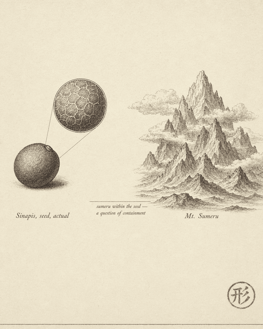

These two passages come from different scriptures, but they share one structural intuition. Indra’s Net says every part mirrors the whole — pick any jewel and you see the entire net. The Sumeru passage says the largest structure fits inside the smallest container without loss — the container’s scale is irrelevant to the content’s structure.
One emphasizes the mapping relationship. The other emphasizes scale-invariance. Together, they outline something precise: the information of the whole is present in every part, and that presence survives changes in scale.
This is not mystical rhetoric. It is a claim about structure — stated in the vocabulary of Buddhist philosophy.
Seventeen hundred years later, a mathematician stumbled into the same territory from a completely different direction.
How long is a coastline?
Lewis Fry Richardson was a British meteorologist with an unusual side interest: he wanted to know whether the length of a shared border between two countries predicted the probability of war between them. When he died in 1961, he left behind unpublished manuscripts containing a strange finding. The same coastline, measured from different data sources, yielded different lengths.
Not measurement error. Something systematic: the finer the ruler, the longer the coast.
Measure the coastline of Britain with a 200-kilometer ruler and you get one number. Switch to a 100-kilometer ruler and you can trace more bays and headlands — the total grows. Use 50 kilometers, and more detail enters the picture. 25, 12, 6 — with each step down, the total length increases, and there is no sign of convergence.
In principle, an infinitely fine ruler would give an infinitely long coastline.
This challenges a deep assumption. We take it for granted that a physical object has a definite length. A table is 1.2 meters. A road is 300 kilometers. These numbers do not change because you swap rulers. But a coastline is different. Its length depends on the precision of measurement, and it does not converge to a limit. “How long is the coast of Britain?” turns out to have no answer within classical measurement.
In 1967, Benoit Mandelbrot published a paper in Science with a title so blunt it bordered on provocation: How Long Is the Coast of Britain? Statistical Self-Similarity and Fractional Dimension. Working from Richardson’s data, he supplied a mathematical framework: the coastline’s length diverges because it is not a smooth one-dimensional curve. Its dimension is a fraction.
The fractal dimension of Britain’s coastline: D ≈ 1.25. More complex than a straight line (dimension 1), but not complex enough to fill a plane (dimension 2). It lives between the two.
Fractal dimension quantifies how thoroughly a shape fills its ambient space — its degree of “roughness” or “crumpledness.” D = 1 is a perfectly smooth line. D = 2 is a completely filled plane. D = 1.25 means the coastline is more complex than a line but falls well short of a surface.
Norway’s coastline has D ≈ 1.52 — the fjords make it far more crinkled, pushing it closer to two dimensions. South Africa’s coastline has D ≈ 1.02 — relatively smooth, barely more than a line.
Dimensions are no longer restricted to whole numbers. That alone is a conceptual breakthrough.
Here is the key insight: the statistical character of a coastline is consistent across scales. The jagged outline you see in a satellite photograph and the jagged outline you see looking down from a cliff at the rocks below your feet are different shapes, but they share the same statistical pattern of jaggedness.
Zoom in and new detail appears. Zoom in again — more detail. Each layer of detail is statistically similar to the layer above.
This is statistical self-similarity: not exact replication, but scale-invariant statistical distribution.
Nature is full of it. River drainage networks, the bronchial tree of a lung, the branching paths of lightning, the silhouette of a mountain range. The pattern you observe at one scale reappears when you shift to another.
But natural self-similarity is approximate, statistical. Is there a shape that is self-similar in the strict, mathematical sense?
The Koch snowflake
In 1904, the Swedish mathematician Helge von Koch constructed a curve.
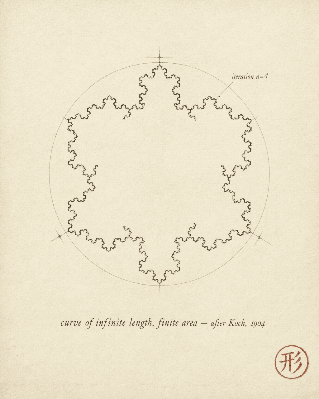
Start with an equilateral triangle. Divide each side into thirds. On the middle third of each side, erect a smaller equilateral triangle pointing outward, then remove the base of that triangle. Each original side has now become four segments, each one-third the length of the original. Repeat the same operation on every new side. And again. And again. Infinitely.
The result is a “snowflake” — its boundary infinitely intricate, every segment a scaled-down copy of the whole.
Two properties make the Koch snowflake a textbook fractal.
Finite area, infinite perimeter. The area increases only slightly with each iteration and converges to 8/5 of the original triangle’s area. But the perimeter multiplies by 4/3 at every step — after infinitely many iterations, it tends to infinity. A shape of finite size whose boundary is infinitely long.
Exact self-similarity. Take any segment of the snowflake’s edge and magnify it by a factor of 3. What you get is identical to the entire edge — not “statistically similar,” but mathematically congruent. The part is a perfect rescaling of the whole.
At each step, every edge segment produces 4 copies of itself, each scaled down by a factor of 3. The fractal dimension is defined as:
where N is the number of self-similar pieces (4) and S is the scaling factor (3):
Nearly identical to the British coastline’s 1.25 — one is a mathematically constructed exact fractal, the other a naturally evolved statistical fractal, yet their dimensions are strikingly close.
The Koch snowflake makes one thing visible: self-similar structure does not require a complicated generator. A single rule — “replace the middle third of every edge with an outward bump” — repeated without end, is enough.
Complexity is not designed. It is iterated. Between the simplicity of the rule and the complexity of the result lies a vast gap, and what bridges it is repetition.
z → z² + c
Take that thought to its limit.
Pick a complex number c. Starting from z = 0, repeatedly compute z → z² + c. If the sequence stays bounded — does not fly off toward infinity — color the point c black. Do this for every point c in the complex plane.
Six characters of rule. The shape they produce is called the Mandelbrot set.
Its boundary is among the most complex shapes known to mathematics. Zoom into any region of that boundary and you find new structure — spirals, tendrils, miniature copies of the set itself. Zoom further, and there is more. Zoom without end, and new detail never stops. And within that detail, variations of the overall shape keep recurring. The part echoes the whole.
Two things are worth pausing on.
First, the Koch snowflake’s rule still involves a geometric operation — “find the middle third, erect a triangle.” The Mandelbrot set’s rule involves no geometry at all. It is pure algebra: square and add. Nobody designed those spirals and tendrils. They are what happens when the same rule acts on itself, over and over.
Second, the Mandelbrot set’s self-similarity is neither the exact congruence of the Koch snowflake nor the purely statistical resemblance of a coastline. It is a subtler third kind: the miniature “baby Mandelbrots” that appear at every scale are recognizably similar to the parent shape but not identical — each carries its own unique decorative detail. Similar, yet not the same. Theme and variation.
Fractals are not designed. They are what emerges when a simple rule is applied to itself repeatedly.
That sentence is worth sitting with. The Koch snowflake is one replacement rule executed without end. The Mandelbrot set is one algebraic rule executed without end. A coastline is the result of waves and geological forces eroding rock at every scale, repeatedly, over millions of years. In all three cases the complexity does not live in the rule — the rule is almost trivially simple. The complexity lives in the accumulation of iteration.
From temple to mathematics
Back to where we started.
The Sumeru-in-a-mustard-seed passage says: the largest structure fits inside the smallest container — scale changes, structure does not. Indra’s Net says: every part mirrors the whole — the whole is present in every part.
The Mandelbrot set says: zoom into any region of the boundary and you find echoes of the overall shape. The Koch snowflake says: take any segment of the edge, magnify it to full size, and it is congruent with the whole.
One is a Buddhist intuition. The other is a mathematical discovery. The paths could not be more different. What they describe is the same structural property: a resonance between part and whole — structural echo.
An honest boundary statement belongs here.
This series is about mental models for agentic systems. We are not claiming that agentic systems are fractals in any mathematical sense — they do not satisfy the formal definition of self-similarity, and they have no precisely computable fractal dimension. This is analogy, not identity.
What we are saying is that the core intuition of fractals — structural echo between part and whole — provides an engineering lens worth looking through. The observe-reason-act loop inside a single agent, the dispatch-execute-aggregate flow at a multi-agent orchestration layer, the emergent coordination patterns across an agent network — when structures at different scales begin to rhyme, that is not coincidence. It is a signal worth investigating.
But before we investigate engineering implications, there is a more fundamental question.
Every fractal we encountered in this article — the Koch snowflake, the Mandelbrot set, a coastline — shares one trait: none of them were designed in a single stroke. Each is the product of a simple rule applied to itself, again and again. Iteration is the generative mechanism.
So what, exactly, is iteration? Under what conditions does the repeated application of a simple rule produce structure — and under what conditions does it produce only noise?
Recursion: the generator of complexity
Self-similarity keeps showing up where nobody invited it. Koch snowflakes and fern leaves. Mandelbrot sets and coastlines. A Buddhist metaphor about Mount Sumeru fitting inside a mustard seed, and a strand of DNA that packs the blueprint of an entire organism into every one of its trillions of cells.
But noticing that self-similarity exists is different from understanding why it exists.
A fern and a snowflake curve are separated by billions of years of evolution and entirely different physics. Why do they converge on the same kind of structure? Self-similarity is not the signature of any single domain — it appears independently in mathematics, biology, and computation, each time without borrowing the pattern from elsewhere. That independence is what makes the question sharp: what mechanism causes self-similar structures to emerge over and over again?
Mathematics: iterated function systems
In 1968, the Hungarian-born botanist Aristid Lindenmayer published a paper in the Journal of Theoretical Biology describing a formal grammar for the growth patterns of filamentous organisms like blue-green algae. His starting point was not geometry — it was developmental biology. He wanted a mathematical language precise enough to express “one cell divides into two, two into four” and nothing more.
The system that emerged, now called the L-system, has a core idea that is almost aggressively simple: take a rule, apply it to its own output, repeat.
An L-system consists of three things: an initial string (the axiom), a set of replacement rules, and an iteration count.
Here is a classic tree-like L-system:
Axiom:   F
Rule:    F → F[+F]F[-F]F
At each step, every F in the string is simultaneously replaced by F[+F]F[-F]F.
The symbols are drawing instructions:
F— draw a line segment forward+— turn left by 25.7°-— turn right by 25.7°[— save the current position and heading (push onto a stack)]— restore the last saved position and heading (pop from the stack)
Step 0: F — a single vertical stroke.
Step 1: F[+F]F[-F]F — a trunk with two short branches splitting left and right.
Step 2: Every F gets replaced again. The string explodes in length — each line segment sprouts its own pair of branches.
By step 4, the string is thousands of characters long. But when you render it, you see a tree with dozens of branching levels. A complete, recognizable tree.
Notice what is absent from the rules: the word “tree.” There is no concept of trunk, canopy, or branch hierarchy. The rule says exactly one thing — “replace each segment with a branching pattern.” The tree is a side effect of iteration, not the goal of design.
Pay attention to what just happened. A single replacement rule, applied to its own output, iterated four or five times, and a visually recognizable tree structure crystallized out of pure string manipulation. The rule contains zero knowledge of trees. No “trunk” variable. No “canopy” parameter. Just “replace F with a branching pattern.” Yet when that rule is recursively applied to its own products, macroscopic structure emerges from microscopic grammar.
Lindenmayer himself probably did not foresee that a grammar invented for blue-green algae would become the standard tool for generating virtual plants in computer graphics. Change the branching angle and the replacement pattern, and the same mechanism produces shrubs, ferns, flowers — all from the same engine: a rule feeding on its own output.
The Mandelbrot set runs on the same logic, just in a different branch of mathematics. Pick a complex number , start with , and iterate:
Track whether escapes to infinity or stays bounded. Different values of lead to different fates — some points flee immediately, some are trapped near the origin forever, some dance along the boundary in extraordinarily intricate trajectories. The set of all values that never escape forms the famous black shape.
One iteration rule. Different initial conditions. The result is a structure that reveals new detail at every magnification. Zoom into the boundary of the Mandelbrot set by a factor of ten thousand, a million, a billion — you do not find pixels and blur. You find new, elaborate patterns that echo the whole. Miniature copies of the full Mandelbrot set are scattered across the boundary, each surrounded by still smaller copies. Five characters — — encode a finite amount of information. But the structure that iteration extracts from them is infinite.
L-systems and the Mandelbrot set come from completely different mathematical traditions — one from formal language theory, the other from complex dynamical systems. Yet they converge on the same conclusion: simple rule + repeated iteration = emergent self-similarity.

There is an important distinction to be honest about here. L-systems produce exact self-similarity — every level of branching is a precise scaled-down copy of the level above, because the replacement rule is identical at every step. Natural plants exhibit statistical self-similarity — the branching angles, length ratios, and branch counts are consistent in their statistical properties across scales, but no two branches are ever identical. An L-system is a mathematical abstraction of plant growth, not a faithful reproduction of it. Real biological systems are buffeted by wind, uneven sunlight, soil nutrient gradients, and competition with neighboring plants — randomness that smears exact self-similarity into the statistical kind. The mathematical model reveals the underlying mechanism; nature adds noise on top.
L-systems appeared in 1968. The Mandelbrot set was first rendered by computer in 1978. A decade apart, from different research traditions, both pointing at the same core mechanism. Mathematics has given its answer: iteration is the generator of self-similarity.
But has nature ever built a real iteration machine — one that has been running for billions of years?
Biology: DNA and cell division
It has. And it is almost as old as life on Earth.
The earliest fossil evidence places cellular life on Earth roughly 3.5 billion years ago. From that point forward, DNA replication coupled with cell division has constituted a recursive engine that has never stopped running. Each time a cell divides, the entire genome is copied and handed to the daughter cell. This process has continued unbroken from the first single-celled organisms to the present moment — the retinal cells you are using to read this sentence, and every cell in your liver, bones, and skin, are all products of approximately 37 trillion divisions descending from a single fertilized egg.
This machine has several structural features worth examining closely.
Every part carries the blueprint of the whole. Each cell in your body (with a handful of exceptions, such as mature red blood cells) carries the complete genome — roughly 3.2 billion base pairs encoding all the information needed to construct the entire organism. A liver cell contains the full instructions for building an eye. A skin cell contains the complete code for assembling a brain. The reason a liver cell is a liver cell and not a neuron is not that it lacks certain information — it is that specific genes have been activated while others have been silenced. The information is complete; the expression is selective.
This is not a metaphor. It is molecular biology. The ancient image of the whole contained within the part — Sumeru in a mustard seed — finds its most literal biological instantiation here.
Encoding consistency across levels. From base pairs to codons, from codons to amino acids, from amino acids to proteins — the encoding mechanism obeys the same grammar at every level. Triplet combinations of four bases (A, T, G, C) translate into twenty amino acids, and this translation table is nearly universal across all known life. Whether the code runs inside E. coli or in a blue whale’s neurons, the codon AUG encodes methionine, and UAA means “stop translating.” The rule does not change with scale. It does not change with species.
A cell is not a passive container. A common misconception treats cells as inert storage devices — biological hard drives waiting to be read. But a single cell is a complete functional unit. It has its own energy metabolism (mitochondria), its own sensory and signaling apparatus (receptor proteins and signal transduction pathways), its own channels for material exchange with the environment (ion channels, endocytosis, exocytosis), and its own quality-control machinery (proteasomes that degrade misfolded proteins). A cell is not a cog in a larger machine — it is itself a complete, independently viable machine. Single-celled organisms proved this point long ago: one cell is one complete life.
Temporal self-similarity. Heredity introduces a dimension that neither L-systems nor Koch snowflakes possess: time. The Koch snowflake’s self-similarity is spatial — zoom in on a portion and you see the same pattern as the whole. An L-system’s self-similarity is across iteration levels — each replacement step produces the same branching motif. But biological heredity’s self-similarity spans generations. Parent and offspring share the same genome. Grandparent and grandchild share the same encoding grammar. Humans and yeast share substantial numbers of homologous genes. Life’s self-similarity is not only “zoom in and see the same pattern” — it is also “at every generation along the time axis, the same fundamental architecture is re-executed.” And that time axis stretches back four billion years.
A clear disclaimer is needed here. Later articles in this series will discuss a structural mapping between the genome and the system prompt — both are “encoded information written into a system before runtime that shapes the system’s subsequent behavior.” But this mapping operates at the structural level, not the mechanistic level. The genome is read and executed by molecular machinery inside the cell — ribosomes, RNA polymerase, spliceosomes — physical entities that are themselves products of the genome but are distinct from it. A prompt, by contrast, is processed by the LLM itself — the same model is both reader and executor. The identity and mechanism of execution are entirely different; only the abstract pattern of “encoded information shaping downstream behavior at system initialization” is shared. Mistaking structural similarity for mechanistic equivalence is one of the most common and most dangerous traps in analogical reasoning.
Mathematics gave us the principle — iteration generates self-similarity. Biology gave us a real-world instance that has been running for four billion years, and this instance exhibits features absent from the mathematical models: every part carrying the complete blueprint of the whole, encoding grammar that is invariant across species, and generational self-similarity along the time axis.
Computation: Conway’s Game of Life
In 1970, Martin Gardner introduced a cellular automaton invented by the British mathematician John Conway in his “Mathematical Games” column in Scientific American. The rules fit on the back of a napkin:
| Condition | Result |
|---|---|
| Live cell, fewer than 2 live neighbors | Dies (underpopulation) |
| Live cell, 2 or 3 live neighbors | Survives |
| Live cell, more than 3 live neighbors | Dies (overcrowding) |
| Dead cell, exactly 3 live neighbors | Becomes alive (reproduction) |
An infinite two-dimensional grid. Each cell is either alive or dead. Every tick, all cells update simultaneously according to those four rules. No player input. No random events injected. No external intervention. Set the initial state, press “go,” and the system evolves on its own.
Start from a random initial configuration and the first few steps look like noise — cells dying and birthing in great swathes with no discernible pattern. But run it for a few dozen steps and something strange begins to happen. Chaos settles. Order condenses out of it.
First come stable static structures: 2x2 blocks, six-cell beehives. Under the B3/S23 rules, they are perfectly balanced — every live cell has exactly two or three live neighbors, so nothing changes. Then come periodic oscillators: the three-in-a-row “blinker” that alternates between horizontal and vertical forever; the “toad” that flips between two states every tick. Nobody designed these structures. They are natural stable solutions that arise wherever local conditions happen to satisfy the rules.
More remarkable still are the moving structures. The “glider” is a pattern of just five live cells that shifts one square diagonally every four ticks, indefinitely. It is not literally sliding — every tick, cells are dying and being born. But after four ticks, the original shape reappears, displaced by one unit. The entire movement is a precisely choreographed sequence of deaths and births, and that choreography is produced entirely by four local rules.
Later, people discovered the “glider gun” — a stable structure that periodically emits gliders. With guns and gliders, you have signal emission and transmission. With signals, you can build logic gates. With logic gates, you can in principle build any computer.
Conway’s Game of Life was subsequently proven to be Turing complete. Four rules about life and death on a two-dimensional grid can, in principle, compute anything that is computable. Paul Rendell’s 2016 monograph Turing Machine Universality of the Game of Life provides the full constructive proof.
But the story does not end there. There is a deeper fact, one directly relevant to self-similarity.
Through an ingenious construction called the OTCA metapixel, roughly two thousand Game of Life cells can be assembled into a “metacell.” The cells inside this metacell obey the standard B3/S23 rules — the same rules as every other cell on the grid. But viewed from a distance, the metacell as a whole behaves exactly like a single Game of Life cell: when exactly three of its neighboring metacells are “alive,” it switches from “dead” to “alive”; when fewer than two or more than three neighbors are alive, it “dies.”
In other words, you can build a Game of Life inside the Game of Life. Each “pixel” in the inner game is not a single grid cell but a vast cluster of cells functioning as a unit — yet from far enough away, it follows the same four rules and produces the same gliders, oscillators, and still lifes. Everything is just a few thousand times larger and a few thousand times slower.
And in theory, the inner Game of Life can use metacells to build yet another Game of Life inside itself. The third layer’s pixels are second-layer metacells, whose pixels are first-layer metacells. Layer after layer, each running the same B3/S23 rules, each producing the same emergent structures. There is no theoretical limit to the depth of nesting.
This is the simplest known instance of “computation within computation.” A system uses its own fundamental elements to construct a complete copy of itself, running the same rules at a larger scale, producing the same emergent behavior.
Three lines converge
Step back and look at the three territories we just visited:
- Mathematics: L-system string replacement rules iterate into tree structures; iterates into the Mandelbrot set. The mechanism is formal. The results are deterministic.
- Biology: DNA replication plus cell division has been iterating for four billion years, producing self-similarity in both space and time. The mechanism is molecular. The results are statistical.
- Computation: Four local rules on a two-dimensional grid iterate into self-organizing structures — and can even reconstruct themselves inside themselves. The mechanism is discrete. The results are emergent.
Three independent domains. Three entirely different substrates — symbolic systems, organic molecules, discrete grids. The same pattern: a simple rule, applied to its own output, executed repeatedly. No master architect required to lay out the global design. No carefully curated initial conditions. No step-by-step human intervention. Just a recursive process running long enough, and complex self-similar structures grow out of simple rules.
This also explains why self-similarity is so pervasive in nature: recursion is nature’s cheapest construction strategy. Encoding a single rule requires far less information than encoding a complete complex structure. Growing complexity through iterated application of a simple rule is orders of magnitude cheaper, in information cost, than designing a complex system from scratch. Natural selection favors economical solutions — which is why a fern grows its shape through recursion rather than describing every leaf pixel-by-pixel in its genome.
But here we must add an honest footnote.
Recursion does not always produce self-similarity. Some recursive systems produce chaos — the Lorenz attractor is driven by three coupled differential equations where each step’s output feeds into the next, which is unambiguously recursive. But its trajectory is exquisitely sensitive to initial conditions; while the overall motion is confined to a butterfly-shaped region, the internal structure does not repeat itself at every scale. Some recursive systems produce uniformity — the heat equation is recursive too (each moment’s temperature distribution is determined by the previous moment’s), but its iteration erases all local differences, converging toward the featureless equilibrium of thermal death. And some recursive systems produce simple periodicity — under certain initial conditions, the logistic map settles into a fixed-point cycle, neither chaotic nor self-similar.
Self-similarity is a common outcome of recursion, but not a guaranteed one. Recursion is a necessary condition, not a sufficient one.
So under what conditions does recursion produce self-similarity? Go back to the three examples and look for what they share.
The answer: self-similarity emerges when the recursive rule maintains structural consistency across levels. The L-system’s replacement rule is identical at every iteration — the first replacement and the hundredth use the same rule — so every level of branching exhibits the same motif. DNA’s encoding grammar is the same in E. coli and in every cell of a blue whale, so every cell carries the blueprint of the whole. The Game of Life’s four rules apply identically to individual grid cells and to entire metacells, so metacells can reproduce single-cell behavior.
Rule invariance across scales — it sounds simple, but it is precisely the critical condition. Remove it and everything changes. Give an L-system a different replacement rule at each level, and the output is no longer a self-similar tree but an unpredictable hybrid.
Cross-scale rule invariance is the true generator of self-similarity.
Fractal dimension: measuring self-similarity
So far, “self-similarity” has been a qualitative description — we say a structure “looks similar at different scales,” but how similar? Is a fern “more” self-similar than a coastline? Is there a ruler that can quantify the property?
There is. It is called fractal dimension.
Recall the British coastline from the previous article: fractal dimension . We said that number means “the coastline’s complexity lies somewhere between one-dimensional and two-dimensional,” but we did not explain where the number comes from.
Imagine covering a geometric object with square boxes of side length , and counting the minimum number of boxes needed to cover it completely. Then shrink the boxes and count again. Repeat, and watch how grows as shrinks.
- If the object is a straight line segment: . Halve the box size, double the count. The signature of a one-dimensional object.
- If the object is a filled square: . Halve the box size, quadruple the count. The signature of a two-dimensional object.
- If the object is a Koch snowflake: . Halve the box size, and the count increases by a factor of about — more than a line, less than a surface.
The fractal dimension is the exponent of that growth rate:
For the Koch snowflake, the dimension can be computed exactly. Each iteration replaces a line segment with 4 segments, each the length of the original (the middle third is replaced by two sides of an equilateral triangle). The self-similarity ratio is , the number of self-similar pieces is , so:
What does for the British coastline mean in practice? It is more complex than a smooth curve () — there is a wealth of detail and irregularity, and halving the measurement scale reveals more than a linear increase in new features. But it is not complex enough to fill an area (). It sits between one dimension and two — at precisely 1.25 dimensions.
The engineering value of fractal dimension is this: it is a cross-domain complexity fingerprint.
The British coastline has . The Koch snowflake has . Nearly identical — yet these two structures come from completely different origins. One is an ideal curve constructed by a mathematician with a deterministic rule. The other is a natural landform sculpted by millions of years of wave erosion and geological process. On the dimension of “how does complexity grow with measurement precision,” they behave almost identically. Fractal dimension maps structurally diverse objects onto a single scale, making cross-domain structural comparison possible.
The branching pattern of a fern and the branching pattern of a river network may share a similar fractal dimension. The frequency fluctuations of a musical signal and the price fluctuations of a stock may share a similar fractal dimension. This does not mean their physical mechanisms are related — ferns do not care about stock prices, and rivers do not follow musical scales. But it does mean that the recursive processes generating these structures share a common abstract property: the degree to which they maintain structural consistency across scales.
That is the real power of fractal dimension as an engineering tool: it does not describe content. It describes the shape of complexity. When you measure similar fractal dimensions in two seemingly unrelated systems, you have a lead worth pursuing — perhaps the generative mechanisms behind them share some structural feature, even if on the surface they have nothing in common. Fractal dimension is a probe for discovering hidden connections, not merely a label for cataloguing known complexity.
From the generator to worlds within worlds
Recursion is the generator of complexity. A simple rule applied repeatedly to its own output, under the right conditions — particularly when the rule remains invariant across scales — produces emergent self-similarity. Mathematics proved it with L-systems and the Mandelbrot set. Biology confirmed it with four billion years of cell division. Computation pushed it to its logical extreme with four rules and a two-dimensional grid — the Game of Life running another Game of Life inside itself.
That last example is worth pausing on.
A system uses its own elements to construct a complete copy of itself, running the same rules at a larger scale, producing the same emergent behavior. This is not merely “the part looks like the whole” — this is the whole being fully re-implemented inside the part. The outer Game of Life has no idea that another Game of Life is running inside it. The inner Game of Life has no idea that each of its pixels is actually a vast colony of cells in the outer game. Two levels, each independently obeying the same rules, each independently producing the same structures.
A world within a world. And the inner world follows the same laws.
This structure — not just resemblance, but complete re-implementation from the inside — is what the next article explores. When recursive nesting goes deep enough, “the part contains the whole” stops being a figure of speech. It becomes an operational engineering fact.
Worlds within worlds
Every cell in your body carries the full genome. Not as an archive — as a live, expressible program. A liver cell holds the complete instructions for building an eye. A skin cell contains the entire blueprint for a heart. They are “liver” or “skin” not because they lack information, but because their environment has activated certain genes and silenced others.
Complete information. Selective expression.
This is worth stopping for. It is not merely a biological fact — it hints at a structural property that keeps surfacing across philosophy, computation, and agent engineering.
The gap
The first article in this chapter observed a phenomenon: structural echo between part and whole. Indra’s Net, Koch snowflakes, the Mandelbrot set — whether the observation came from Buddhist philosophy or twentieth-century mathematics, it pointed at the same thing. Zoom into a part, and you see the shape of the whole.
The second article asked where that echo comes from. The answer was recursion — a simple rule applied to its own output, repeatedly, with structural consistency across scales. That is the generator.
But there is a gap between “the part looks like the whole” and “the part is the whole.”
A segment of the Koch snowflake’s edge is a scaled-down copy of the entire edge. Geometrically perfect self-similarity. But that segment does not do anything on its own. It has no internal state, no causal chain, no capacity to evolve independently. It is a geometric fragment that happens to resemble its parent shape.
A cell is different. A cell does not merely look like an organism — it carries the complete information to build one, and it is itself a fully operational system. Place a cell in a petri dish with the right culture medium and it survives, metabolizes, divides. It is not a component. It is a complete world.
This article is about the far side of that gap: not just parts that resemble wholes, but parts that constitute complete, independently viable worlds — worlds that follow the same structural laws as the whole they are embedded in.
The gold lion
In the seventh century, the Tang dynasty monk Fazang faced a pedagogical problem. He needed to explain Huayan Buddhism’s central claim — that each part of reality contains the totality — to Empress Wu Zetian, who was not a philosopher. He pointed to a golden lion statue in the palace.
Gold has no inherent form; it follows the craftsman’s skill and manifests as the lion’s shape. The lion’s form is empty — it is nothing but gold. … Take any single hair-pore of the lion: it contains the entire lion. Every hair-pore is likewise.
Gold, as a substance, has no fixed shape — it takes the form of a lion only because a craftsman made it so. The lion’s shape is “empty,” meaning not that it does not exist, but that it is not a separate entity independent of the gold. Form and substance are inseparable. Then the critical move: pick any single hair-pore on the lion’s body, and that pore contains the entire lion. Every pore does.

This is not a claim about visual resemblance — the pore does not look like a tiny lion. Fazang’s point is that the gold in the pore and the gold of the whole lion are the same gold. Structure and substrate cannot be separated. The part does not “map to” the whole. The part is the whole, expressed at a different position and scale.
Fazang was the third patriarch of the Huayan school, and his contribution was to take the poetic imagery of the Avatamsaka Sutra — Indra’s Net, the interpenetration of all phenomena — and formalize it into a systematic philosophical framework. Francis Cook’s Hua-yen Buddhism (1977) remains the standard English-language study of this tradition for readers who want the full philosophical architecture.
“One is all, all is one” — a line from the Avatamsaka Sutra that is often treated as Zen-flavored mysticism. In Fazang’s systematic reading, it is a precise structural description: every part contains sufficient information to reconstruct the whole, and the whole is nothing other than the simultaneous expression of all its parts.
A thousand years later, an English poet arrived at nearly the same intuition through entirely different means.
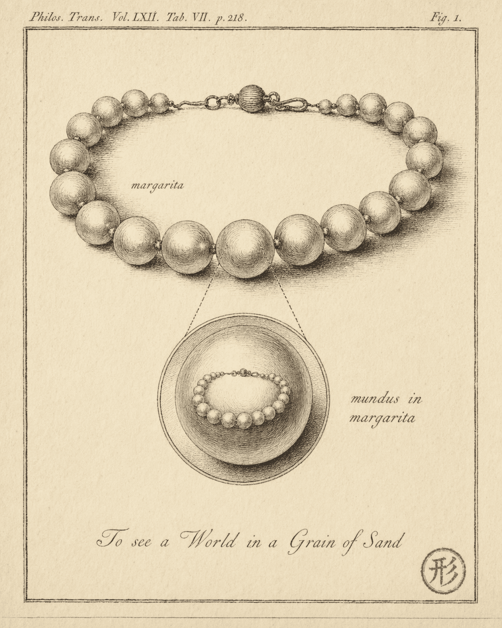
To see a world in a grain of sand, And a heaven in a wild flower, Hold infinity in the palm of your hand, And eternity in an hour.
A world in a grain of sand. Not “a grain of sand reminds you of a world” — the grain is a world. The logic is structurally identical to Fazang’s hair-pore argument: the part contains enough structure to constitute a complete, self-consistent existence.
These philosophical intuitions grew independently across cultures separated by a millennium and half the planet. Fazang never read Blake. Blake almost certainly never read the Avatamsaka Sutra. Yet they converge on the same structural insight: the part does not merely mirror the whole — the part is itself a complete world.
The genome in every cell
Philosophical intuition is one thing. Molecular biology is another.
The human body contains roughly 37 trillion cells. Every one of them — with rare exceptions like mature red blood cells, which eject their nuclei — carries the complete genome: approximately 3.2 billion base pairs encoding all the information needed to build the entire organism.
But cells do not merely store this information passively. That is the critical point.
A stem cell carries the full genome. When it receives signals from its environment — chemical gradients, physical contact, molecular messages from neighboring cells — its gene expression profile shifts. Certain genes activate. Others go silent. Same blueprint, different context, different outcome:
- Near the neural tube, a stem cell differentiates into a neuron — expressing ion channel proteins, extending axons and dendrites, acquiring the ability to conduct electrical signals.
- In bone marrow, a stem cell differentiates into a red blood cell — massively upregulating hemoglobin production, eventually ejecting its own nucleus to make room for more oxygen cargo.
- Near muscle tissue, a stem cell differentiates into a muscle fiber — expressing actin and myosin, gaining the capacity to contract.
The same complete information. Different contexts. Entirely different functions.
This pattern has a direct structural counterpart in agent engineering: the same agent architecture — same model, same core capabilities — configured with different system prompts and tool sets, exhibiting entirely different behaviors. One agent architecture can be a code reviewer, a document writer, a data analyst. What determines its function is the “environment” — the signals you place around it.
An explicit disclaimer belongs here: this is a structural mapping, not a mechanistic equivalence.
The genome is read by molecular machinery inside the cell — ribosomes translate mRNA into proteins, RNA polymerase transcribes DNA into RNA, spliceosomes edit pre-mRNA. These molecular machines are themselves encoded by the genome, but they are physically distinct from it. The “reader” and the “blueprint” are two different things.
A system prompt, by contrast, is processed by the LLM itself. The same model is both reader and executor. Reader and blueprint collapse into one.
What the two systems share is an abstract pattern: encoded information, written into a system at initialization, selectively expressed through interaction with the environment, shaping the system’s functional specialization. This pattern is real and testable. But if you mistake structural similarity for mechanistic equivalence — if you conclude that a system prompt “is” a digital genome, or that a tool set “is” epigenetic regulation — you have slipped from a useful analogy into a false equation.
Simulations within simulations
In 2003, the philosopher Nick Bostrom published “Are We Living in a Computer Simulation?” in the Philosophical Quarterly. The paper’s conclusion is a trilemma — three propositions of which at least one must be true. We do not need to evaluate whether the conclusion is correct. What matters here is its premise structure.
Bostrom’s reasoning rests on an assumption: if a sufficiently advanced civilization has enough computational resources, it could simulate a complete universe containing conscious beings. And the civilization inside that simulation, if it develops sufficient technology, could run another simulation inside its own reality.
Strip away the debates about consciousness and probability, and what remains is a purely structural claim: computation can nest. A complete computational system can run inside another computational system, and the inner system need not be aware of the outer one.
This is not a thought experiment. Conway’s Game of Life already provides the minimal implementation.
The OTCA metapixel uses roughly two thousand Game of Life cells to construct a single “metacell.” The cells inside this metacell follow the standard B3/S23 rules — exactly the same rules as every other cell on the grid. But observed from a distance, the metacell as a whole behaves exactly like a single Game of Life cell. Tile enough metacells together and you have a complete Game of Life running at a larger scale inside the original Game of Life.
The inner “world” is complete for its inner “inhabitants.” It has its own rules (B3/S23 — the same as the outer layer, though the inner layer does not need to “know” this). It has its own state (the on/off pattern of metacells). It has its own causal chains (inner-layer gliders and oscillators evolve according to inner-layer dynamics). The inner world does not need to know that the outer world exists. It is a self-consistent, complete system.
Here is the key property: the completeness of the inner world does not depend on awareness of the outer world. You do not need to know you are inside a simulation to run a complete causal chain within that simulation. Completeness is structural — it depends on whether the rules are sufficient to support self-consistent evolution, not on whether you know where the rules came from.
Agents creating sub-agents: world construction
Back to engineering.
When an agent creates a sub-agent, what is it doing?
On the surface: delegating a task. But structurally, it is doing something more interesting. It is constructing a complete world.
- System prompt — the physical laws of this world. It defines what is permitted, what matters, where the boundaries are.
- Tool set — the interactive environment. Whatever the sub-agent can “touch” constitutes its reality.
- Task description — the purpose of this world’s existence. It gives the sub-agent a direction, an answer to “why am I here.”
- Context — the initial state. The sub-agent begins its existence from this information.
The sub-agent runs inside this world. It observes (reads context and tool outputs), decides (generates next tokens), acts (calls tools), verifies (checks feedback). A complete perceive-decide-act loop. Then the world closes, and the results pass back to the creator.
The critical point: the sub-agent does not know, and does not need to know, the orchestrator’s full context.
The orchestrator might be managing ten sub-agents simultaneously, each handling a different subtask. A given sub-agent sees only its own system prompt, its own tool set, its own task description. It does not know it is “the third one created.” It does not know the other nine exist. It does not know the orchestrator’s ultimate goal. For the sub-agent, its world is the entirety of what exists.
This is structurally identical to the metacell Game of Life. The inner layer does not know about the outer layer. The inner layer has its own complete rules and causal chains. The inner layer’s “completeness” is structural — it depends on whether the system prompt defines a clear behavioral space and whether the tool set supports task execution, not on whether the sub-agent “knows” the orchestrator’s full picture.
Between 2025 and 2026, this structure appeared independently across major agent products. Claude Code’s primary agent can spawn sub-agents, each with its own system prompt and tool permission set distinct from the primary agent’s configuration. OpenAI’s Codex shipped subagent capabilities at general availability in March 2026, allowing agents to dynamically create child agents at runtime. Devin’s multi-step workflows exhibit structurally similar nesting patterns.
Did these products borrow design ideas from each other? Possibly — or possibly not. Public information does not settle the question. But regardless of each team’s design process, the structure they converged on is strikingly similar: an orchestrator constructs a complete runtime environment for a sub-agent, the sub-agent runs independently within it, and upon completion returns its results.
Structural convergence is often more telling than any individual designer’s intent.
Pattern unification
Four domains. One structure.
| Domain | ”Whole" | "Part” | What the part contains | Can the part run independently? |
|---|---|---|---|---|
| Huayan philosophy | Indra’s Net | A single jewel | Complete image of the entire net | Each jewel is a complete world |
| Biology | Organism | A single cell | Complete genome | Yes — survives in a petri dish |
| Computation | Outer Game of Life | Metacell inner layer | Complete B3/S23 rule set | Yes — evolves independently |
| Agent engineering | Orchestrator | Sub-agent | System prompt + tools + task | Yes — testable in isolation |
These four rows do not describe four things that “sort of look alike.” They share a testable structural property: a part contains sufficient information to constitute a complete, independently viable functional world.
“Testable” is not rhetorical. It implies a concrete test:
Extract the part from the whole. Can it run on its own?
- A cell can. Remove a cell from an organism, place it in a petri dish with appropriate culture medium, and it survives, metabolizes, divides. The entire existence of single-celled organisms is proof of this.
- A metacell inner-layer Game of Life can. Extract the inner layer’s initial state, run it in a standalone simulator under B3/S23 rules, and its evolution is identical to what it would have been inside the outer layer.
- A sub-agent can. Extract its system prompt, tool set, and task description, launch it in an independent agent runtime, and it executes its task without needing the orchestrator to exist.
If a “part” fails this test — if it cannot function when separated from the “whole” — then what you have is not a world within a world. It is a component. Components can have self-similar shapes, but they lack independent causal chains, their own “physical laws,” their own standing as a “world.”
A segment of the Koch snowflake’s edge is a component. It looks like the whole, but extract it and nothing happens. It has no state, no evolution, no timeline of its own.
Cells, metacells, and sub-agents are worlds. Each possesses complete operational rules, independently evolvable state, and self-consistent causal chains. They do not merely resemble their parent wholes — each one is a whole, nested inside another.
This “part as complete world” property is not a one-time invention by a single mind. It appears independently in nature, philosophy, and computation.
What is more telling is that engineers are independently reinventing it — not because they read the Avatamsaka Sutra or studied OTCA metapixels, but because in the process of solving real problems, this structure keeps proving itself effective.
That is not coincidence. When entirely separate domains converge on the same structure without cross-referencing each other, it usually means the structure reflects a constraint that transcends any single domain — something about how complex systems manage information across scales.
The next article looks at how engineers arrived at this structure on their own.
From transistor to agent
Engineers keep reinventing the same structure. Not because they read Mandelbrot or studied fern branching patterns. Most of them did not know each other’s work. But when the complexity of a problem outgrows the capacity of a single component, they converge, again and again, on the same solution: decompose the system into smaller copies of itself, have each copy honor the same interface contract, and glue them together with a thin coordination layer.
This is not a catalog of parallel examples. It is an evolutionary line, from switches etched in silicon to agents reasoning in natural language. The abstraction rises with each step; the structural pattern stays put.
Hardware: transistor to multi-core (1947–2005)
The story starts at the bottom.
A transistor is the smallest computational unit: voltage in, state flip, voltage out. On or off. 0 or 1. In 1947, Bardeen, Brattain, and Shockley at Bell Labs built the first working point-contact transistor. Its entire repertoire was a controlled switch, but that switch is the atomic operation underneath all digital computation.
Organize a few billion transistors and you get a CPU core. Inside the core runs a fetch-decode-execute cycle: pull an instruction from memory, decode what it means, execute the arithmetic, write back the result. Input, transform, output. The same logic as the transistor, lifted one abstraction level. A transistor flips a single bit; a core completes an entire instruction in a single clock tick.
In 2005, Intel shipped the Pentium D, its first commercial dual-core processor. The timing was not accidental. Single-core clock frequencies had hit a power wall. Dennard scaling broke down, and pushing frequency further meant melting the chip. Engineers did not respond by building a “bigger core.” They put N identical cores on the same die. Each core runs its own independent fetch-decode-execute loop; a cache coherence protocol coordinates shared state between them.
Stop on that choice for a moment. Faced with “one unit is not enough,” the engineering instinct was not to redesign the unit. It was to replicate the unit and add a coordination layer. Multi-core is not a bigger core. It is N copies of the same structure plus a protocol. This pattern will recur.
In 1967, Gene Amdahl pointed out a constraint that sounds obvious once stated and is routinely underestimated in practice: the speedup of a program is bounded by the fraction that cannot be parallelized. If 10% of the work must run sequentially, the theoretical speedup ceiling is 10x, no matter how many cores you throw at it.
where is the parallelizable fraction and is the number of cores. As , .
The intuition is blunt: parallelism cannot rescue you from your serial bottleneck. Double your cores from 64 to 128, and if only 90% of the workload is parallelizable, your theoretical speedup goes from 8.8x to 9.3x. Diminishing returns set in hard.
This structural constraint does not predict anything about agent systems directly. CPUs execute deterministic instructions; agents execute probabilistic reasoning. But the shape of the constraint echoes forward: in any system that decomposes work into parallel sub-units, the parts that resist decomposition become the binding constraint on the whole. We will hear this echo again.
In a multi-core system, each core has its own L1/L2 cache. When core A modifies a cache line, core B’s copy of that line is now stale. B must invalidate it and re-fetch from shared cache or main memory. The MESI protocol (Modified, Exclusive, Shared, Invalid) maintains this consistency through bus broadcasts.
More cores mean more invalidation broadcasts. This is why consumer processors rarely exceed 16 cores: coordination overhead eventually eats the gains from parallelism.
The pattern, “coordination cost grows non-linearly with participant count,” has a structural echo in agent systems. But the analogy has a hard boundary that must be marked honestly. A cache line is deterministic. An address is either valid or invalid; there is no in-between. An agent’s state is probabilistic: two agents’ “understanding” of the same codebase can overlap, contradict, or be partially correct at the same time. The structural shape rhymes. The implementation mechanics are fundamentally different.
The operating system layer discussed in the previous chapter manages exactly this level of the fractal. Multiple cores each run identical execution loops; the OS scheduler decides which process runs on which core, and context switches save and restore each core’s register state. Hardware provides self-similar compute units; the OS provides the mechanism that coordinates them.
Software: Unix pipes (1978)
The hardware fractal was forced into existence by physics. The power wall blocked frequency scaling and engineers had no alternative. The next fractal is different. It was deliberately designed.
In 1978, Doug McIlroy, E. N. Pinson, and B. A. Tague published an article in the Bell System Technical Journal (volume 57, issue 6) that laid out the Unix design philosophy. This was not a post-hoc summary. It was the theoretical crystallization of design decisions behind an operating system that had already been running for nearly a decade. The central principle: each program does one thing well, and the output of one program can become the input of another.
A single command:
grep "error" server.logstdin in, processing, stdout out. Same shape as a transistor. Same shape as a CPU core. Input, transform, output.
Chain them with pipes:
grep "error" server.log | sort | uniq -c | sort -rn | head -20Five commands, each honoring the stdin-to-stdout contract. The pipe connects one output to the next input. The whole pipeline, viewed from outside? Still stdin to stdout.
Wrap the pipeline in a shell script:
#!/bin/bash
# top_errors.sh
grep "error" "$1" | sort | uniq -c | sort -rn | head -20
This script’s external interface? stdin to stdout. It can be called by another script, piped into another pipeline, scheduled by cron. The consumer does not need to know whether it is a one-liner or a thousand-line Python program inside.
Four scales (single command, pipeline, script, composition of scripts), one interface contract.
The power of Unix does not come from any individual command being powerful. grep is not powerful. sort is not powerful. uniq is not powerful. The power comes from interface consistency: because every component obeys the same contract (text flows in, text flows out), any component can freely compose with any other. The result of composition still obeys the same contract, so the result can be composed again.
This is the algebraic property of closure: the result of an operation remains in the same set and can therefore participate in further operations. Integer addition yields an integer, so you can keep adding. A Unix command’s output is a text stream, so you can keep piping. The real force of a self-similar structure is not the capability at any single level. It is the composability between levels.
And this self-similarity was designed and enforced as social contract. McIlroy and his colleagues did not stumble into the pattern. They wrote it down as design principle and used it to vet every new tool admitted to the system. Any program that violated the stdin/stdout contract was considered a second-class Unix citizen. Unlike multi-core’s self-similarity (which physics forced into being), Unix’s self-similarity required voluntary compliance from every developer to sustain.
Frontend: Cycle.js — the self-conscious fractal (2015–2016)
From transistors to Unix, self-similar structure kept showing up in engineering, but always implicitly. The engineers designing multi-core processors did not say “we are building a fractal.” The programmers writing shell scripts did not say “we are maintaining self-similarity.” It was just “good engineering.” Everyone did it; nobody named it.
Then, in 2015, someone named it. André Staltz, in an article comparing unidirectional data flow architectures, offered a precise definition that gave engineers a vocabulary for enforcing the pattern deliberately rather than stumbling into it:
“A unidirectional architecture is said to be fractal if subcomponents are structured in the same way as the whole is.”
Cycle.js, the framework Staltz created, is the direct embodiment of this definition. Every component is a pure function: it receives sources (input streams) and returns sinks (output streams). The entire application’s signature is sources → sinks. Each sub-component inside the application? sources → sinks. Sub-components inside sub-components? Still sources → sinks.
A year later, Anton Telesh built on this foundation and formalized four rules for fractal architecture:
- Unified interface — the application is a tree of components sharing the same API
- Recursive composition — every component can contain other components
- No privileged root — the top-level component is structurally identical to a leaf component
- Glue separated from logic — assembly code lives outside the component tree
Look back at those four rules and check them against Unix pipes. Unix satisfies three out of four: unified interface (stdin/stdout), recursive composition (pipelines nest inside scripts), glue separated from logic (the shell handles piping, programs handle data). The one it misses is “no privileged root.” Unix’s init process (PID 1) is genuinely special: it cannot be killed and does not follow normal process lifecycle rules.
What shifted between Unix and Cycle.js was not the pattern but the awareness. Unix is an implicit fractal. Cycle.js is an explicit, self-conscious one. A concept moved from unnamed practice to named principle. And that move from doing it to knowing you are doing it matters for engineering: once engineers recognize the fractal structure, they can deliberately maintain it, propagate it, and enforce it as a design constraint. Staltz and Telesh turned a tacit engineering intuition into an explicit architectural rule.
Agent systems: 2025–2026 convergence
Then, between 2025 and 2026, the same pattern surfaced in a completely new domain. Not on silicon, not in terminals, not in browsers, but in LLM-powered agent systems.
Claude Code’s architecture includes a component called AgentTool. When the main agent determines that a task needs isolated context or parallel processing, it can spawn a sub-agent. What does that sub-agent run? A complete agent loop: gather context, take action, verify result, repeat. Structurally identical to the main agent’s loop, operating on a narrower task slice with independent context. The sub-agent has the same tool set, the same permission model, the same reasoning capability. It is not a stripped-down executor. It is a full agent.
One detail: the sub-agent cannot spawn sub-agents of its own. This is a deliberate termination condition. Recursion needs a base case, or it becomes infinite recursion. L-systems have iteration depth limits, Game of Life metacells are bounded by computational resources, and Claude Code uses permission constraints to achieve the same function. Every recursive system needs a “stop here” mechanism.
In March 2026, OpenAI’s Codex reached general availability with sub-agent capabilities. A manager agent decomposes a task and distributes it to worker sub-agents; each worker runs the same reasoning loop: gather context, execute actions, verify results, decide whether to continue. Like Claude Code’s AgentTool, each worker is a structurally complete agent, not a diminished executor.
Devin 2.0 took a slightly different path. Multiple full agent instances run in parallel inside isolated virtual machines, coordinated by an orchestration layer. Each instance runs a complete agent loop with its own filesystem, terminal, and browser. The orchestration layer manages task allocation and result aggregation between instances, not the reasoning process inside them.
These products developed structurally similar architectures across 2025–2026. Whether there was direct mutual influence between them is unclear, and beside the point. What matters is the fact itself: when the complexity threshold of “a single agent is not enough” arrived, recursive decomposition was the answer engineers independently converged on.
Why recursive decomposition and not some other approach? Because the alternatives are harder. You can build a “bigger agent” with a longer context window and stronger single-pass reasoning, but that road has physical limits; context windows cap out, and single-pass reliability degrades with task complexity. You can also build a fundamentally different architecture, a central dispatcher paired with reasoning-free executors. That throws away the strongest capability LLMs offer: every node can reason and make decisions autonomously. Recursive decomposition keeps recurring because it simultaneously preserves the unit’s full capability and the system’s scalability.
This is the same story as Unix inventing pipes when “a single command is not enough” and Intel choosing multi-core when “a single core is not enough.” Different motivations, different constraints, same destination.
One evolutionary line
Pull the thread out and lay it flat:
| Era | Domain | Base unit | Structure | Coordination mechanism |
|---|---|---|---|---|
| 1947 | Hardware | Transistor | Input → state flip → output | Circuit wiring |
| 2005 | Hardware | CPU core | N × fetch-decode-execute | Cache coherence (MESI) |
| 1978 | OS | Unix command | stdin → process → stdout | Pipe | |
| 2015 | Frontend | Cycle.js component | sources → sinks | Framework driver layer |
| 2025–2026 | AI | Agent | context → action → verify → loop | Orchestration / permission constraints |
The timeline is not perfectly linear. Unix predates multi-core by nearly three decades. But the abstraction level rises monotonically: from electrical signals to instruction pipelines, to text streams, to reactive data flows, to natural-language-driven reasoning loops.
Each step’s designers faced different problems, worked with different materials, operated under different constraints. But they independently arrived at the same architectural pattern: decompose the system into structurally identical sub-units, compose freely through a uniform interface, manage inter-unit state consistency through a coordination mechanism.
This is not coincidence. It is the engineering-side validation of the conclusion from the second article in this chapter.
That article found the same pattern across mathematics, biology, and computation: recursion is the default generator of complexity. A simple rule applied repeatedly to its own output, with structural consistency maintained across scales, produces self-similar structure. The evolutionary line from transistor to agent says the same thing with the perspective inverted. Not “recursion naturally produces self-similarity,” but “engineers solving complexity problems naturally reach for recursion.” L-system rewriting rules do not know they are generating fractals. McIlroy did not know he was designing fractal architecture. Claude Code’s development team did not know they were replaying the Unix pattern. Yet all of them arrived at the same structure, because decomposing a whole into structurally identical parts, letting each part run independently, and coordinating through a shared protocol is the most natural way to manage complexity.
But every row in that table hides an unexpanded word: “coordination.” Transistors use wiring. Multi-core uses MESI broadcasts. Unix uses pipe buffers. Agents use orchestration layers. The coordination mechanism exists at every level, and at every level it is the dominant source of system complexity.
Amdahl’s law says: the serial bottleneck determines the scaling ceiling. MESI says: coordination cost grows non-linearly with participant count. A full Unix pipe buffer blocks upstream. An agent orchestration layer’s context window has a length limit. These constraints did not vanish as the abstraction level rose. They only changed form: from a physical power wall to an informational coordination wall.
Fractal structure gives engineers a powerful tool for managing complexity. But this tool is itself subject to a set of structural limits. What are those limits, and under what conditions do they start to bite?
Where the fractal breaks
Coordination cost exists at every level. Transistors pay it in wiring. Multi-core chips pay it in cache coherence broadcasts. Unix processes pay it in pipe buffers. Agents pay it in orchestration layers. The abstraction rises; the overhead never disappears — it just changes costume.
If the previous four articles left you with a comfortable feeling that one model explains everything, this article’s job is to take some of that comfort back. Not because the fractal model is wrong, but because it is a skeleton — and a skeleton tells you where the structure repeats without telling you how different the physics is at each level.
Where a model stops working is as informative as where it works. The four dimensions ahead — latency, cost, coordination, fault tolerance — are not arbitrary engineering headaches. They share a single root cause: fractals describe structural self-similarity, but the runtime physics at each level is qualitatively different.
Latency: multiplication, not scaling
Geometric fractals scale without changing their properties. Zoom into a stretch of coastline and the roughness looks the same. Zoom into a branch of the Koch snowflake and you see the same snowflake. Scale changes; properties do not. That is the core promise of mathematical fractals.
In agent systems, “scale” has a time dimension, and what happens along that dimension is not scaling. It is a qualitative shift.
A single prompt call typically completes in the range of hundreds of milliseconds to a few seconds — depending on model size, input length, and infrastructure. This is the time scale of the atomic operation, structurally analogous to the transistor’s nanosecond flip: one smallest unit completing one full cycle.
An agent loop — gather context, act, verify, repeat — generally runs for several to a dozen or so iterations, pushing total latency into the tens-of-seconds-to-minutes range. Notice the relationship: it is not “one call plus a little overhead.” It is N calls, each with its own context assembly, model inference, and result parsing.
A multi-agent system — several agents running their own loops, plus information exchange between them — pushes latency into the minutes-and-beyond range. Even when workers run in parallel, the orchestrator’s synthesis step remains serial: wait for all workers to return, parse each result, build the global picture, decide the next move. Parallelism shrinks the worker layer’s latency but does not eliminate the orchestrator’s serial bottleneck.
Every handoff between agents carries a non-zero cost. One handoff means: one API call’s network round-trip, one context window assembled and filled, one result parsed and validated. If the worker’s output does not meet expectations, add retry and clarification overhead. Each of these costs is modest in isolation, but they are multiplicative — each additional layer of collaboration does not add a constant to latency, it multiplies by a coefficient.
Geometric fractals maintain self-similarity across scales because their recursion consumes no time. The Koch snowflake from the first iteration to the hundredth is purely a descriptive unfolding, not a physical process. Agent recursion is a physical process — every layer of unfolding consumes real time, and the time consumed grows with depth. On the time axis, the fractal’s promise of “infinite nesting” starts showing its price at the third or fourth layer: user patience is finite, task deadlines are real, and the world may have changed while the system was thinking.
Cost: superlinear growth
Latency you can wait out. Tokens cost money.
A single agent’s token consumption has two main components: input (system prompt + context + user instructions) and output (reasoning + tool calls + result generation). When you decompose one agent into an orchestrator plus several workers, token consumption does not simply get distributed — the orchestrator must understand the full task to decompose it, each worker must understand its subtask to execute it, and then the orchestrator must understand every worker’s return to synthesize a result.
The source of superlinearity matters. Suppose a task is split into three subtasks, one per worker. The orchestrator spends tokens understanding the original task and generating a decomposition plan. Three workers each spend tokens understanding their subtask and executing it. Then the orchestrator spends more tokens understanding three separate results and synthesizing a final output. There is substantial redundant “understanding” — the orchestrator comprehends the full task twice (once to decompose, once to synthesize), and each worker re-ingests whatever context it needs from scratch. In a single-agent architecture, that redundant comprehension cost simply does not exist.
Engineering experience consistently shows that multi-agent systems consume several times — and sometimes an order of magnitude more — the tokens of an equivalently complex single-agent approach. The exact multiplier depends on task nature, decomposition strategy, and context management quality, but the direction is unambiguous: superlinear growth.
Here is a property that true fractals do not have: lossy compression. When a worker agent finishes its subtask, it cannot return its entire reasoning trace to the orchestrator — that would overflow the orchestrator’s context window. It returns a summary, a compressed result. That compression is lossy. Details are discarded, and the orchestrator has no way to know whether the discarded details were critical.
Mathematical fractal recursion involves no information loss. Each iteration of the Mandelbrot set, , is exact — no rounding, no omission, no “summary.” Agent recursion is inherently lossy. Structure repeats, but information decays at every cross-layer handoff.
There is also a hard constraint: the context window. Mathematical fractals have no “canvas size” limitation — you can zoom in forever, nest infinitely, with no “we’ve run out of space” problem. Every agent’s context window is finite. This finiteness is not merely a storage limit — it determines how much information the agent can process, how deep a conversation it can sustain, how complex a coordination task it can manage. More subtly, even before the window physically overflows, the model’s attention to earlier information degrades as context grows longer. The context window is not just a hard wall — it is a floor that gradually softens, where older information stands on increasingly shaky ground.
Fractal recursion can go infinitely deep. Agent recursion is truncated by a finite, degrading canvas.
Coordination: zero to O(n²)
Coordination cost is the most structural of these boundaries, because it directly governs how wide a system can scale.
A single prompt call has zero coordination cost. One request, one response, nothing to synchronize. This is the simplest case — a closed input-output process with no other participants.
A single agent loop has implicit coordination — the context window itself serves as shared state. Each step’s output becomes the next step’s input, requiring no explicit synchronization protocol. The context window plays the role of shared memory, and only one “thread” accesses it, so there are no race conditions. Coordination is free, but only because there is a single participant.
Multi-agent collaboration pushes coordination from implicit to explicit. The orchestrator must track each worker’s status. Workers may need to share intermediate results. Task dependencies must be managed explicitly. In the worst case, pairwise communication channels among N agents scale as O(n²) — each additional participant adds not one new link but N-1. Even the hub-and-spoke topology of an orchestrator pattern only simplifies this to O(n) at the center, and that center itself becomes a bottleneck: the orchestrator must “understand” each worker’s output, and “understanding” in the LLM context means putting output into a context window and reasoning over it, which consumes tokens and time. As the orchestrator’s context fills up, reasoning quality degrades — a subtle but real bottleneck.
The observable engineering pattern: diminishing returns arrive quickly as agent count grows. Going from one to three workers usually yields clear improvements in task quality and speed — each worker handles an independent subtask, and the orchestrator’s synthesis burden remains manageable. From three to ten, improvement becomes uncertain — some tasks benefit from finer decomposition, others actually degrade as orchestrator synthesis load increases. Beyond that range, coordination cost tends to consume whatever gains parallelism provides. Amdahl’s law echoes clearly: the orchestrator’s synthesis step is a serial bottleneck, and no number of parallel workers makes it disappear.
This is not a new story. The MESI protocol’s dilemma from the previous article echoes here — more cores mean more cache coherence broadcasts, which is why consumer processors rarely exceed sixteen cores. Agent systems face the same class of problem in a different medium. But the medium matters: MESI broadcasts precise cache line states — Modified, Exclusive, Shared, Invalid — four states, zero ambiguity. Agents exchange natural language — a summary, an instruction, a result. Natural language coordination is orders of magnitude less precise than bus-level broadcast, which means coordination failure is orders of magnitude more likely. The same structural constraint, at a higher abstraction level, manifests more severely, not more leniently.
Fault tolerance: errors amplify, not attenuate
In conventional software, a failed component does something identifiable. It throws an exception, returns an error code, or crashes outright. The signal is unambiguous: something went wrong here. Downstream components can catch the exception, check the error code, or be restarted by a watchdog. Errors are discrete, recognizable events.
Agent failure looks nothing like this. An agent that makes a reasoning error — misunderstanding the task, calling the wrong tool, drawing the wrong conclusion — does not throw an exception. It produces a perfectly plausible-looking output: grammatically correct, logically coherent, properly formatted, and wrong. The error does not arrive as an “exception.” It arrives dressed as a correct answer.
When that output reaches a downstream agent, the downstream agent has no built-in mechanism to distinguish “this is valid input” from “this is upstream’s mistake.” There is no error code to check, no exception to catch, no CRC checksum to verify. There is only a stretch of natural language, and natural language has no “semantic checksum.” The downstream agent treats the flawed output as reliable input, builds new reasoning on top of it, and potentially compounds the error — because it is constructing a reasoning chain on a contaminated foundation.
This is error cascade: errors propagate across layers without attenuating — they amplify. Traditional software’s error propagation model rests on an assumption of independence: each step faces correct preconditions, faults are independent events, and total failure probability is the product of individual step failure probabilities. In agent systems, that independence assumption breaks. The previous step’s error changes the problem the next step faces. One agent corrupts a function signature; the downstream agent calling that function encounters an interface that “looks reasonable but is semantically wrong.” It is not merely at risk of its own independent error — it has been steered toward error by the upstream mistake. This is coupled amplification, not independent accumulation.
The fractal structure means nesting: outer layers contain inner layers, and inner layers’ outputs become outer layers’ inputs. In this structure, error amplification is not an incidental bug — it is a structural risk. The deeper the nesting, the more amplification steps an error passes through before reaching the outermost layer. And the amplification is particularly insidious: unlike conventional software, which announces failure loudly through exceptions and error codes, agent errors travel between layers quietly, wearing the disguise of correct output, accumulating and mutating as they go. By the time the outermost layer notices something is wrong, the cost of tracing back through layers of plausible-looking output to find the source is already steep.
Mathematical fractal recursion is exact — each step’s output faithfully becomes the next step’s input; ‘s precision carries forward to . Agent fractal recursion is probabilistic — each step can introduce deviation without issuing any warning, and that deviation will be treated as fact by every step that follows.
Simon’s correction: near-decomposability
Four boundaries are now on the table: latency undergoes qualitative change, cost grows superlinearly, coordination explodes, errors amplify. Do these boundaries mean the fractal model should be discarded?
No. They mean it needs a correction term — a framework that explains why structure repeats but runtime physics does not.
In 1962, Herbert Simon published The Architecture of Complexity and introduced a concept he called near-decomposability. Simon was not studying fractals. He was asking a more basic question: why do complex systems almost always exhibit hierarchical structure? His answer was evolutionary pressure — his watchmaker parable demonstrated that systems assembled from stable subcomponents survive evolutionary selection far more readily than systems with no intermediate structure.
These hierarchical systems share a common property — interactions within a subsystem are much stronger than interactions between subsystems. Strong, but not absolute isolation; weak, but not complete independence. The word “near” in “near-decomposable” carries all the nuance. Full decomposability would mean zero inter-subsystem interaction — just a collection of unrelated systems that happen to sit next to each other. Full indecomposability would mean all components interacting at equal strength with no discernible subsystem boundaries — an impenetrable tangle of complexity. Nearly every complex system worth studying falls between these extremes.
Simon also identified a key dynamic property: frequency separation. Dynamics within a subsystem are high-frequency — fast-changing, locally scoped. Dynamics between subsystems are low-frequency — slow-changing, interacting through aggregated outputs. You do not need to know every part’s state inside another subsystem; you only need its aggregate output.
Map this framework onto agent systems:
- Within a single agent, dynamics are high-frequency — each gather-act-verify step iterates rapidly, internal state changes constantly
- Between agents, dynamics are low-frequency — the orchestrator does not need to know every reasoning step inside a worker, only its final output (the aggregate)
- In the short term, each agent can run approximately independently — this is the structural precondition that makes parallelization viable
- Long-term behavior emerges through aggregate interfaces — the system’s overall performance surfaces through the interaction of aggregated outputs, not through the sum of internal agent states
This frequency separation is not merely descriptive — it has design implications. If different levels of a system operate at different speeds, then using the same coordination strategy for all levels is a mismatch. High-frequency inner iteration needs lightweight, low-latency coordination (implicit state sharing within a context window is sufficient). Low-frequency outer interaction needs structured, verifiable coordination (aggregate summaries, typed interfaces, explicit state confirmation). Applying high-frequency strategies to low-frequency layers — say, having the orchestrator track every reasoning step of every worker in real time — is waste. Applying low-frequency strategies to high-frequency layers — say, requiring a formal structured report at every single iteration step — is a bottleneck.
The fractal model says: structure repeats across levels. Simon’s near-decomposability adds: although structure repeats, runtime physics at different levels is heterogeneous. Inner layers are fast, outer layers slow. Inner layers are tightly coupled, outer layers loosely coupled. Inner layers are high-frequency, outer layers low-frequency.
Agent systems are structurally fractal — the same input → process → output pattern repeats at every level. But at runtime, they are level-heterogeneous — latency, cost, coordination complexity, and fault tolerance characteristics undergo qualitative change at each level. The fractal describes the skeleton. Near-decomposability describes the muscle and blood.
Looking back at the four boundaries through Simon’s framework, they receive a unified explanation:
- Latency undergoes qualitative change — because dynamic processes at different levels run on different time scales; inner high-frequency iteration and outer low-frequency synthesis are naturally out of tempo
- Cost grows superlinearly — because inter-level communication in a near-decomposable system is aggregative, and aggregation means compression, and compression means information loss and extra overhead
- Coordination explodes — because inter-level interactions are weak but not negligible, and maintaining those weak interactions costs more as participant count grows
- Errors amplify — because aggregate outputs discard internal detail, and downstream cannot distinguish correct aggregation from erroneous aggregation
These four boundaries are not four independent engineering problems. They are four projections of one structural fact: the fractal describes the skeleton, but each layer of that skeleton operates under different physical conditions.
This correction does not weaken the fractal model. It does the opposite — it delimits the model’s scope of applicability, turning it from a metaphor that “sounds elegant but who knows how to use it” into an analytical tool with boundary conditions.
Boundaries as freedom
Latency multiplies across levels, which makes the synchronous-versus-asynchronous character of inter-level interaction a structural variable. When a layer blocks on another layer’s line-by-line progress, it inherits that layer’s full latency chain.
Coordination cost grows nonlinearly with participant count. This gives agent count a structural ceiling — there is a point past which adding participants costs more in coordination than it returns in parallelism.
Errors amplify across levels rather than attenuating, which means inter-level boundaries carry a verification burden. The cost of checking an output before it crosses a boundary is structurally lower than the cost of tracing an error that has been amplified through three layers of reasoning.
These boundaries are the fractal model’s preconditions for engineering use. A map that marks cliffs and marshes is not telling you “don’t travel.” It is telling you which paths are clear and where you need different equipment. A map that omits the cliffs is not a more optimistic map — it is a more dangerous one.
Each of the four boundaries does the same thing: it reshapes the fractal from an idealized model of infinite recursion into a practical model of finite layers. Latency sets the depth limit. Cost sets the resource budget per layer. Coordination complexity sets the parallel width within a layer. Fault tolerance sets the trust model between layers. Together, these four dimensions sculpt “infinite self-similarity” into “constrained self-similarity.”
These boundaries define the operating envelope — they tell you the depth, width, and trust budget available at each layer.
The fractal gave us a skeleton. Near-decomposability gave each layer its own physics. Boundary conditions gave us engineering constraints. These three, layered together, form the complete picture. So within those constraints — what does the fractal structure actually give the engineer? What is the payoff?
The dao of fractals
From analysis to understanding
Five articles, one structure examined from different angles.
The first was intuition: part and whole share a structural echo. The second was mechanism: a simple rule applied to its own output generates self-similarity. The third went deeper, arguing that each level is not merely similar to the whole but is a complete world running the same logic. The fourth was historical evidence: engineers across decades and domains, working independently, converged on the same architecture. The fifth was honest constraint, mapping where latency, cost, coordination explosion, and failure propagation break the model.
That was analysis — facts about the structure. Understanding is different: once the structure is internalized, certain insights surface on their own. You see a property at one layer and already sense what the adjacent layers look like. What follows is what emerges when fractal structure shifts from an external concept to an internalized lens.
Cross-layer principle migration
Anthropic’s Building Effective Agents contains an observation:
“Think about your tools […] tool descriptions deserve just as much prompt engineering attention as your overall prompts.”
Tool descriptions deserve the same care as system prompts. This is a finding at the prompt layer — write tool descriptions well and the agent selects tools more accurately. Most readers nod, file it under “prompt engineering tips,” and move on.
With fractal structure internalized, that observation does not stay at the “tool” layer. It unfolds across levels in your mind, not because you deliberately extrapolate, but because you have already seen three layers sharing the same skeleton. The observation stops being an isolated tip about tools and becomes one layer’s projection of a principle.
Three layers (prompt, agent, swarm) share the same skeleton: input description, comprehension, decision, execution. That was the conclusion of the third article: each level is not just analogous to the whole; it is a complete world running the same logic. If “description quality determines comprehension quality” holds at the prompt layer, it holds at the agent and swarm layers too. Not because someone ran the experiment at each level, but because the structure is the same.
At the agent layer: an orchestrator needs to know what each sub-agent can do before it can assign work correctly. A sub-agent’s capability description and a tool description are structurally the same thing, both interface contracts that let a higher level understand a lower level’s competence boundary. Vague capability descriptions cause the orchestrator to misroute tasks, the same way vague tool descriptions cause an agent to pick the wrong tool.
At the swarm layer: the task description an orchestrator hands down to a sub-agent is structurally equivalent to a system prompt. Both define the behavioral boundaries of an executor. Ambiguous task descriptions degrade sub-agent output quality the same way ambiguous system prompts degrade model output quality.
Notice what happened. There were no three independent analyses, no separate data collection at each layer, no three white papers. One principle was understood carefully at one layer, then mapped along the self-similar structure to neighboring layers — and the mapping held, because the skeleton is the same.
This is the first cognitive payoff of fractal structure: cross-layer principle migration. When you discover an effective principle at one layer, you do not need to rediscover it. Check the corresponding structure at adjacent layers; if the skeleton matches, the principle transfers directly. Cognitive load drops from “think independently at every layer” to “think deeply at one layer, then map.” The reverse holds too: if a problem at one layer resists solution, look one layer up or down. The isomorphic problem may already have been solved somewhere else.
The base case in recursive decomposition
Fractals are recursive. But engineering recursion faces a hard constraint that mathematical recursion does not: it must terminate.
A Koch snowflake can iterate forever. Mathematics charges no compute fees, and nothing collapses if the millionth iteration draws a segment slightly wrong. Engineering systems do not get that deal. Each additional layer of recursion adds latency, consumes tokens, and extends the call chain that might break. Recursion without a termination condition is called infinity in mathematics and disaster in engineering.
Claude Code’s sub-agent architecture has a quiet but telling design choice: a sub-agent cannot spawn further sub-agents. The AgentTool is unavailable inside the child process. That is the base case. Recursive decomposition stops at this layer, and the remaining work is completed by a single prompt call.
This is not an arbitrary restriction. Without a base case: an agent decomposes a task and hands pieces to sub-agents; a sub-agent decides the piece is still too complex and decomposes further; the chain extends with no bound. Every layer adds a network round-trip and consumes a full context window. Errors at any depth can propagate upward. And when something goes wrong, you are debugging a call chain whose depth you do not even know.
So any recursive decomposition has a termination layer — a layer where problems are executed directly, not delegated further. That termination layer is typically a single prompt call: input specific enough, output clear enough, no further splitting needed.
The base case does not negate fractal structure. It depends on it. Precisely because each layer is a complete world (the third article’s conclusion), the base-case agent can finish its task independently, without further decomposition. Self-similarity guarantees the base case’s self-sufficiency: a sub-agent receiving a sufficiently concrete task has the same reasoning capabilities, tool access, and input-process-output loop as the top-level agent. It is not a degraded agent. It is a full agent with a narrower scope.
When does recursion terminate? A natural signal: when the task description is already concrete enough to complete in a single prompt interaction, further decomposition no longer reduces complexity — it only adds coordination overhead. This is not a precise boundary; it shifts with model capability, context length, and task nature. But the question itself — “does further splitting still reduce complexity?” — is a stable anchor for judgment.
Inter-layer decoupling: Simon operationalized
The fifth article introduced Simon’s near-decomposability: strong interaction within subsystems, weak but non-zero interaction between them. In that article it served as a theoretical lens. Overlay it on fractal structure and a more concrete picture comes into focus.
In a fractal system, each layer is a complete world. Components within a layer share the same context window (or the same state space), tightly coupled to each other, and correctly so. An agent’s multi-step reasoning shares a single conversation history; within a sub-agent’s task execution, one step’s output directly feeds the next. Intra-layer coupling is a prerequisite for functioning. Weaken it and every step rebuilds context from scratch.
Between layers, the opposite. When a Claude Code sub-agent finishes its task, it returns a text summary, not the full context window. The AgentTool does not inject the child process’s entire conversation history into the parent. It performs deliberate information compression. A sub-agent may have gone through ten tool calls, three error corrections, two strategy pivots, but what flows upward is the final conclusion and key findings only.
This “lossy compression” is near-decomposability realized in fractal architecture. Inter-layer interaction is not zero; the orchestrator does need to know what the sub-agent accomplished. But the granularity of that interaction is deliberately coarsened: not a step-by-step transcript but an aggregated summary. Simon’s phrase, “the short-run behavior of each component subsystem is approximately independent” while long-run interactions occur “only in an aggregate manner,” has an almost literal engineering counterpart here.
Why lossy? Return to the coordination cost analysis from the fifth article. If complete information flowed between layers, with every sub-agent’s full context injected into the orchestrator, coordination cost would grow nonlinearly with participant count, O(n^2) information exchange. When sub-agents scale from two to five, the orchestrator’s context window floods with lower-layer detail, and the attention budget remaining for its own decisions shrinks sharply.
Why not lossless? Because not all information is relevant to the upper layer’s decisions. The specific syntax errors a sub-agent encountered, the alternative paths it tried, the tool invocation details: these are high-frequency intra-layer dynamics with no bearing on the low-frequency inter-layer decisions. Compressing them away is noise filtering, not information loss.
Intra-layer high coupling for execution efficiency. Inter-layer low coupling (lossy compression) for coordination cost control. These are not independent principles but two faces of the same structural property, near-decomposability, showing up in a fractal system.
Simon described near-decomposability in 1962 using examples from physical systems and social organizations. Six decades later, the same structural property reappears in agent systems in nearly unmodified form. If fractal structure genuinely preserves self-similarity across scales, this is expected: the properties that constrain fractal structure hold across scales too. Near-decomposability was not “applied to” agent systems. It is what comes bundled with the architecture.
Fractal fitness test
The three insights above, cross-layer migration, base case, inter-layer decoupling, all surfaced naturally from fractal structure. But how do you tell whether a given system actually has good fractal properties?
Two questions are enough.
1. Can a design principle learned at level N apply, without modification, at level N+1?
This tests self-similarity. If an effective principle at the prompt layer stops working at the agent layer, the structural skeleton has fractured between those two levels. A fracture is not necessarily an error; it may be a deliberate design choice (the base case intentionally terminates recursion). But if it is not deliberate, it is worth investigating.
2. Can a component at level N serve as an atomic unit at level N+1?
This tests composability. Can an agent be invoked by an orchestrator as a black-box capability, the same way the agent invokes a tool? If the upper layer needs to understand the lower layer’s internals to use it correctly, composability is broken. What you have is not a fractal but a tangle.
Two “yes” answers: the system has good self-similarity and composability; cross-layer principle migration is likely to work.
One “no”: locate the fracture point and determine whether it is intentional design (like a base case) or accidental coupling leakage.
These two questions are diagnostic instruments, not dogma. Not every system needs fractal properties, and not every absence of fractality is a problem.
A counterexample: some systems face fundamentally different constraints at different layers. Latency dominates at the bottom, cost dominates at the top. In that situation, design principles should differ between layers; the first question yields “no,” and that “no” is correct. The diagnostic’s value is not in chasing two “yes” answers. It is in this: when the answer is “no,” you can articulate why, and you know whether that fracture point was placed there on purpose.
Their real use: when a complex system leaves you disoriented, these two questions locate structural inconsistencies fast. Then you decide what those inconsistencies mean.
Orthogonality and fractals
Orthogonality tells you the direction of force. Given that model capability keeps growing, where should your engineering investment point? Direction right, investment compounds. Direction wrong, investment erodes.
Fractals tell you the texture of structure. When a system repeats the same skeleton at different scales, understanding one layer is understanding all of them. The cognitive payoff is dimensionality reduction: not independent thinking at every layer, but deep thinking at one layer followed by structural correspondence checks at adjacent layers.
Direction and structure. These two dimensions are themselves orthogonal. Knowing where to apply force tells you nothing about what the system looks like. Seeing the system’s structure tells you nothing about which investments are worth making. Each provides information independently; together they cover more cognitive ground than either one alone.
And this orthogonal relationship can itself be verified by the fractal fitness test. Orthogonality as a principle holds at the prompt layer (choosing the direction of prompt investment), at the agent layer (choosing the direction of harness engineering investment), and at the swarm layer (choosing the direction of architectural investment). One mental model passing another mental model’s diagnostic. This consistency was not engineered into the two models. It falls out of the fact that both describe properties of the same underlying system.
Direction and structure are two coordinate axes for understanding agentic systems. But the coordinate system is not yet complete — there are other dimensions waiting to be identified.